Geoscience Reference
In-Depth Information
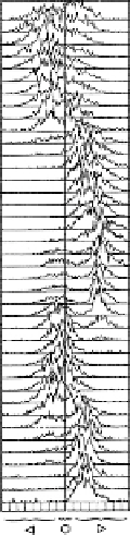
ST. CROIX 8/22/33
Doppler velocity (m/sec)
(Range of 251.3 kms)
Distance (kms)
2
300
2
150
0
150 300
8
9 0 1 2 3 4
1
300
22:06:00
0
2300
22:07:00
1
300
0
22:08:00
2
300
1300
22:09:00
0
2
300
1
300
22:10:00
0
22:11:00
2
300
1300
0
22:12:00
2300
1
300
22:13:00
0
2300
22:14:00
22:10
22:15 22:20
August 22, 1983
(a)
22:25
22:30
(b)
Figure 6.30c
Examples of square waves in the Doppler velocity using gray scale (to
the left) and spectra plots (middle). The plots on the right are interferometric velocities
across the beam. A range of 250 km corresponding to 105 km altitude. [After Riggin et al.
(1986). reproduced with permission of the American Geophysical Union.]
show next is typical) would enter the field of view at a range that decreases with
time, even if it was unstable at a fixed height.
Various observations have implied that
E
s
layers tend to organize into frontal
structures with phase fronts aligned northwest to southeast (northeast to south-
west) in the Northern (Southern) Hemisphere. Sinno et al. (1965) analyzed time-
delay measurements of Loran transmissions in the Northern Hemisphere and
concluded that they could be explained by an organization of
E
s
layer plasma
into frontal structures with the orientation described. Goodwin and Summers
(1970) came to a similar conclusion by analyzing data from a spaced ionosonde
network in the Southern Hemisphere. Goodwin (1966) suggested that the fronts
could be 1000 km long. Bowman (1989) modeled scintillations from
E
s
layers
in the Southern Hemisphere as opaque high-density strips arranged in a frontal
structure, also with the alignment described. The fact that the frontal alignment
mirrors about the equator suggests an electrodynamic cause.


Search WWH ::

Custom Search