Geoscience Reference
In-Depth Information
February 17-18, 1976
B
z
(SM)
10
5
Jicamarca
Mapped from Chatanika
a
10
4
10
10
3
AU
AL
b
500
10
2
Mid-latitude
Horizontal mag field
10
1
10
8
c
50
10
7
Westward
Auroral E-field
10
10
6
d
0
2
10
10
5
0.5
0
e
10
4
B
Z
Trivandrum
Eastward
EQ. E-field
20.5
10
3
0.01
0.1
1
10
16
20
00
04
08
12
Frequency (cycles/hour)
(b)
UT
(a)
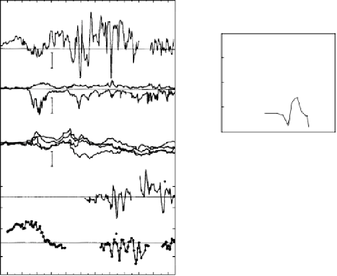
Figure 3.25
(a) Interplanetary (
B
z
), auroral (AU, AL), and midlatitude magnetic field
data along with auroral and equatorial electric field data during a series of rapid interplan-
etary magnetic field changes. [After Gonzales et al. (1979). Reproduced with permission
of the American Geophysical Union.] (b) Power spectra of the data plotted in (a). The
Chatanika electric field data were reduced by the factor
L
3
/
2
before analysis to show
the value that would arise in the equatorial plane at
L
5
R
e
. [After Earle and Kelley
(1987). Reproduced with permission of the American Geophysical Union.]
=
5
.
and magnetic field data (from India and the interplanetary region) are plotted in
Fig. 3.25b and are very similar. The daytime poleward magnetic field data from
India were 180
◦
out of phase with the nighttime eastward electric field data. The
same anticorrelation on opposite sides of the earth was shown recently by Kelley
et al. (2007). The anticorrelation of Indian poleward magnetic field and Peruvian
eastward electric field data shows that when the electric field perturbation is east-
ward at night it is westward during the day. Control of the earth's low-latitude
electric field fromhundreds of thousands of kilometers away in the interplanetary
medium is indeed remarkable. The auroral zone data (from Chatanika, Alaska)
were mapped to the equatorial plane before the Fourier analysis was done so
that they could be directly compared to the Jicamarca data (which are also in


Search WWH ::

Custom Search