Geoscience Reference
In-Depth Information
a)
Observed variation
Correct
Model
Objective functions
Location (
X
)
Low
High
Correct solution
Z
T
X
T
P
T
Ideal convergence path
Source
b)
Z
=
Z
T
Correct solution
P
Location (
X
)
P
T
X
Location (
X
)
Location (
X
)
X
T
c)
P
=
P
T
Z
Correct solution
Z
T
Location (
X
)
Location (
X
)
X
T
X
Location (
X
)
Location (
X
)
d)
X
=
X
T
P
Location (
X
)
Location (
X
)
P
T
Correct solution
Z
T
Z
Location (
X
)
Location (
X
)
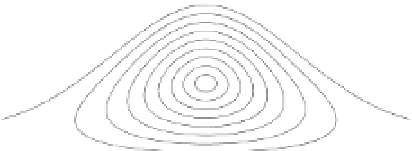
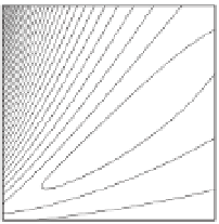
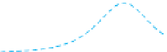
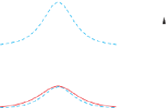
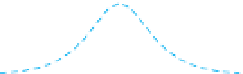
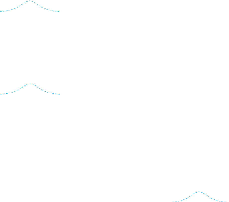
Figure 2.48
Illustration of geophysical inversion based on the gradient of the objective function. (a) Data from a traverse across a body with a
positive contrast in some physical property. The inversion seeks the true location of the source (XT,
T
,Z
T
) and the true physical property contrast
(
Δ
P
T
). (b) Inversion constrained by setting depth (Z) equal to Z
T
whilst the lateral position (X) and physical property contrast (
Δ
P) are allowed
to vary. The objective function shows a single minimum coinciding with the correct values XT
T
and
Δ
P
T
. Also shown are the observed and
computed responses for selected pairs of X and
P
T
whilst X and Z are allowed to vary.
Again, the objective function has a simple form with a single minimum. (d) Inversion constrained by setting X equal to X
T
whilst Z and
P. (c) Inversion constrained by setting
P equal to
Δ
Δ
Δ
P are
Δ
allowed to vary. In this case, the ability to balance variations in
P and Z between each other produces a broad valley of low values in the
Δ
objective function. Note that the inverse problem is greatly simpli
ed when there are only three variables, one of which is held constant and set
to the correct value, whilst the other two are allowed to vary.


Search WWH ::

Custom Search