Geophysical data acquisition, processing and interpretation - Geophysics for the Mineral Exploration Geoscientist - page 42

a)

x

Moving window
P 1

y n+2

P 2 P 3

y

y n+1

P x , y +1

P 4 P 5 P 6

P Output

P 7 P 8 P 9

y n

P x -1, y P x +1, y

Data
points

y n-1

P x , y -1

Contours

Total horizontal
gradient

y n-2

x n-2 x n-1 x n x n+1 x n+2

P Output = function ( P 1 , P 2 , P 3 , P 4 , P 5 , P 6 , P 7 , P 8 , P 9 )

b)

Total horizontal
gradient

( P / y )

( P / r)

Figure 2.23 Convolution in 2D with a 3 3 filter kernel. See text
for details.

( P / x )

The results of convolution can also be obtained with
Fourier operations. The convolution of a filter series with
a data series is equivalent to filtering in the frequency
domain ( Fig. 2.21 ) , as described in Transforms above.

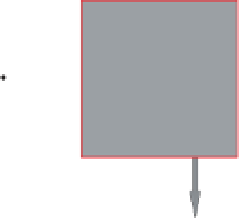
Figure 2.24 Calculation of horizontal gradients. (a) Calculation
of horizontal gradients (derivatives) of gridded data based on
differences between adjacent grid nodes. See text for details.
(b) The total horizontal gradient is the vector sum of the horizontal
gradients in the X and Y directions and is everywhere perpendicular
to contours of the data.

2.7.4.4 Common filters
We demonstrate some of the more commonly used filters
on a 1D data series containing a variety of features mim-
icking the common types of signals and noise encountered
in mineral geophysics ( Fig. 2.25 ). The input series includes
random variations, abrupt discontinuities and spikes
(common types of noise) and smooth variations with vari-
ous wavelengths. Depending on the objectives of the
filtering, the variations of different wavelength may be
considered as either signal or noise.

across-line direction as the Y-derivative ( y). They are the

horizontal gradients of the measured parameter. For some
types of geophysical data, it is also possible to compute the
vertical gradient, or Z-derivative (

∂ P/ ∂

z), which shows how
the measured parameter changes as the distance to the source
(survey height) changes. The vertical gradient, unlike the
horizontal gradients, has the advantage of responding to
changes irrespective of the orientation of their source with
respect to the survey line. These three derivatives are the first
derivatives in their respective directions.
Derivative filters can be enacted in the spatial and fre-
quency domains. A 2D spatial domain derivative

P/

∂ ∂

Gradients and curvature
In Section 2.2.3 we described the measurement of gradients
of a physical property field. Some of the gradients can also be
computed from the survey data, and enhancements obtained
in this way are the most common form of

lter
is illustrated in Fig. 2.24a ; the derivative of the gridded
dataset of P is approximated as the gradient at the location
(x n , y n ). The gradients in the X and Y directions are
obtained from the differences in values at adjacent grid
nodes, spaced

filtering used to
assist interpretation of geophysical data. Gradient or deriva-
tive filters resolve variations in the geophysical response with
distance, with time, or with frequency. The results are usu-
ally referred to as derivatives. The term derivative (from
calculus) refers to the gradient of continuous functions
whose data samples are in nitesimally close, so the gradient
of discretely sampled data approximates the derivative; but
in geophysics the terms are used synonymously.
For a parameter (P) acquired along parallel lines, gradients
of the measured field determined in the along-line direction
are referred to as the X-derivative (

x in the X direction and y in the Y

Δ Δ

direction, using the expressions:

P ð x n + 1 , y n Þ P ð x n 1 , y n Þ

∂ P

∂

x ð

x n , y n Þ≈ ð 2 : 2 Þ

2 x

Δ

P ð x n , y n + 1 Þ P ð x n , y n 1 Þ

∂ P

∂ y ð

x n y n Þ≈ ð 2 : 3 Þ

,

2 Δ y

They can be implemented as a convolution (see Convolu-
tion above), each gradient kernel being {1/2, 0, P/ x), and those in the - 1/2}.

∂ ∂