Geoscience Reference
In-Depth Information
a)
0
1
Survey
lines
Kilometre
A
B
10
A
A
20
b)
c)
Olympic Dam Breccia Complex
Data points
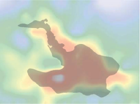
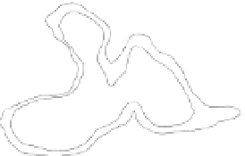
Figure 2.18
Circular anomalies produced by the minimum
curvature gridding illustrated in contours of IP-phase response
(where IP
induced polarisation), at a constant pseudo-depth,
from the Olympic Dam IOCG deposit in South Australia. Positive
(A) and negative (B) circular anomalies are caused by inadequate
sampling of the anomalous areas. Based on a diagram and data
from Esdale et al.(
2003
).
¼
compromise is to select a cell size of between 1/5 and 1/3
the line spacing. A smaller cell size can only be justi
ed by
having closer sampled data, and in particular closer survey
lines.
Even with these cell sizes, interpolation in the across-line
direction can be a challenge for gridding algorithms. Lat-
erally continuous short-wavelength anomalies, as might be
associated with a steeply dipping stratigraphic horizon or a
dyke, can cause particular problems. The phenomenon is
variously referred to as beading, boudinage, steps, step
ladders, string of beads, etc. The aeromagnetic data in
Fig. 2.17
illustrate the effect. Note how the individual beads
have dimensions in the across-line direction equal to the
line spacing, allowing this kind of artefact to be easily
recognised. As the anomaly trend approaches the survey
line direction, individual beads become more elongated
towards this direction.
A problem with minimum curvature algorithms (see
Section 2.7.2
)
is their tendency to produce round
anomalies, often referred to as bulls-eye anomalies. This
occurs because an unconstrained minimum curvature sur-
face is a sphere. Where data points are sparse and the true
shapes of features not properly de
ned by the data sam-
pling,
0
10
Kilometres
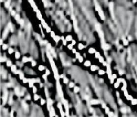
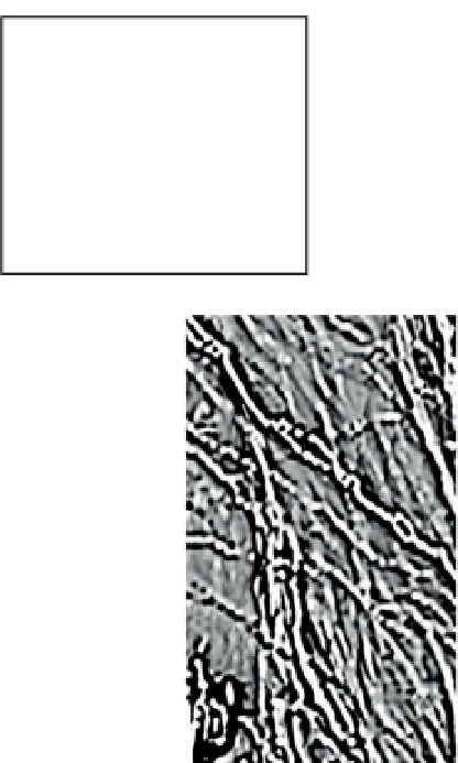
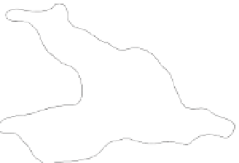
Figure 2.17
Beading in gridded data containing elongate anomalies.
The example is aeromagnetic data from South Australia. (a) Close-
up of beaded data showing how each bead is centred on a survey line.
(b) Data gridded using the inverse-square technique with minimum
curvature applied. The rectangle is the area shown in (a). (c) The
same data gridded using a trend-enhancement algorithm. Data
reproduced courtesy of Department of Manufacturing, Innovation,
Trade, Resources and Energy, South Australia.
that make up the gridded data and may cause artefacts to
appear along the join of the different datasets.
When the data to be gridded consist of parallel lines,
with station spacing much smaller than the line spacing,
the cell size must account for the anisotropic distribution
of the measurements. It is not uncommon for the across-
line sampling interval to be greater than the along-line
interval by a factor of 50 or more in reconnaissance
surveys, with 1:10 or 1:20 common for detailed prospect-
scale surveys. A cell size based on the along-line sampling
interval will create major dif
culties for interpolation in
the perpendicular direction, potentially creating artefacts
(see below). On the other hand, choosing a cell size based
on the line spacing will result in the loss of a lot of valuable
information contained in the line direction. The normal
the gridding algorithm makes
them circular
(
Fig. 2.18
).
Both beading and bulls-eyes are the result of inadequate
sampling by the survey. The solution is more measure-
ments, but this may be impractical. The problem can be


Search WWH ::

Custom Search