Geophysical data acquisition, processing and interpretation - Geophysics for the Mineral Exploration Geoscientist - page 30

a) e)

Anomaly maximum > 1800 nT

Anomaly maximum > 8000 nT

b) f)

Anomaly maximum > 1800 nT Anomaly maximum > 8000 nT

c) g)

Anomaly maximum > 2900 nT Anomaly maximum > 8000 nT

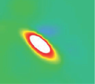
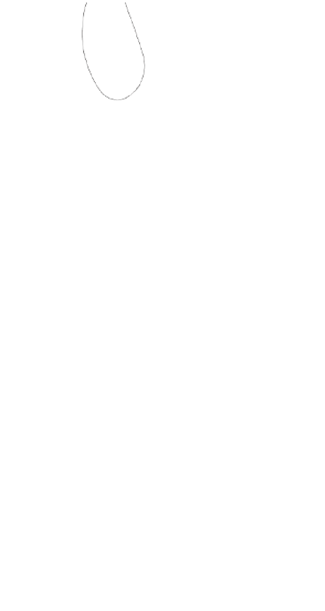
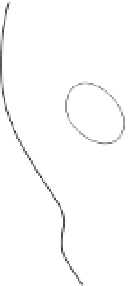
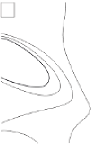
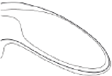
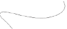
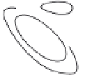
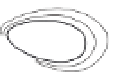
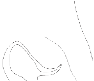
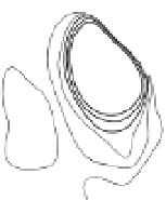
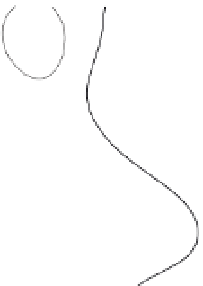
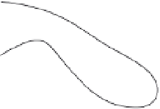
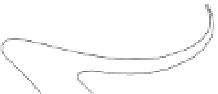
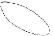
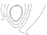
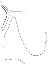
Figure 2.12 Aeromagnetic data from the Marmora Fe
deposit. The gridded, imaged and contoured data were
created from various subsets of the full dataset to
demonstrate the effects of survey line spacing and position
on anomaly resolution. The contour interval is variable.
(a)

d) h)

(d) Line spacing is 1,600 m, with the lines progressively
laterally shifted 400 m in each case. (e)

-

(h) Line spacing
progressively decreased by 400 m, with the central line
optimally located directly over the deposit: (e) 1,600 m,
(f) 1,200 m, (g) 800 m, (h) 400 m. Note the spectacular
improvement in every aspect of the anomaly, i.e. its
amplitude, shape, gradients and trend direction, with
optimally positioned lines and decreasing line spacing.
TMI

-

Anomaly maximum > 8000 nT Anomaly maximum > 8000 nT

4000

0 1
Kilometre

TMI
(nT)

Survey lines

total magnetic intensity. Based on diagrams in
Agocs ( 1955 ) .

-

500

a range of station and line intervals ( Fig. 2.10d ) . Here a
small area has been surveyed with greater detail, as would
be required to characterise a target (see Section 2.6.1 ).
Multiple surveys of differing speci

An uneven spatial distribution of samples can lead to
aliasing (see Section 2.6.1 ) . Figure 2.10 shows several survey
con gurations with uneven sampling. In these cases the

degree of aliasing will vary with location and, in line-based
con gurations, with survey line orientation. The smaller
along-line

cations and extent are
a common occurrence and can provide useful information
for designing subsequent surveys. sampling interval allows short-wavelength