Geoscience Reference
In-Depth Information
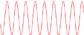
a)
Min
eralisa
tion
Time
Sampling frequency > 2
f
In
25 m Station spacing
250 nT
0.25 m Station spacing
Sampling frequency =
f
In
0.25 m Station spacing
(filtered)
Min
eralisa
tion
Sampling frequency <
f
In
0
200
400
600
800
1000
Location (m)
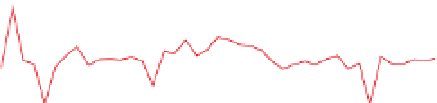
Figure 2.9
Aliasing in total magnetic intensity data across the Elura
Zn
Ag massive sulphide deposit. See text for details. Redrawn
from Smith and Pridmore (
1989
), with permission of J. M. Stanley,
formerly Director, Geophysical Research Institute, University of
New England, Australia.
-
Pb
-
Sample
Input waveform
Waveform after sampling
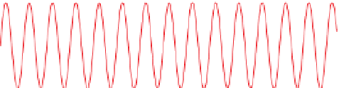
b)
Output
frequency
(Hz)
are under-sampled and converted (aliased) to spurious
lower-frequency signals,
Under-sampled
into
the Nyquist interval. The aliased responses mix with the
responses of interest and the two are indistinguishable. The
aliased responses are artefacts, being purely a product of
the interaction between the sampling scheme and the
waveform being sampled.
The sampling interval required to avoid aliasing can be
established with computer modelling (see
Section 2.11
)
,
reconnaissance surveys or
i.e. they are
'
folded back
'
100
50
0
0
50
100
150
200
250
300
350
400
Input frequency (
f
In
)
(Hz)
Nyquist
interval
Nyquist
frequency
(
f
N
)
Sampling
frequency
(
f
S
)
field tests conducted prior to
the actual survey. In practice, economic and logistical
considerations mean that aliased data are often, and
unavoidably, acquired. This is not necessarily a problem
for qualitative interpretations such as geological mapping
or target detection. Regions with similar characteristics will
usually retain apparently similar appearance even if alias-
ing has occurred, but different geology will give rise to
different geophysical responses. Extreme caution is
required when the data are to be quantitatively analysed,
i.e. modelled (see
Section 2.11.3
)
, because working with an
aliased dataset will result in an erroneous interpretation.
Figure 2.8
Aliasing of a periodic signal of frequency f
In
. (a) Signal
and various sampling frequencies; see text for explanation. (b) The
relationship between the frequency of the input signal and the
frequency of the sampled output signal for a sampling frequency of,
say, 200 Hz. Note how under-sampling causes the output to
'
fold-
back
'
into the Nyquist interval (0
-
100 Hz), e.g. an input signal of
250 Hz produces a sampled output signal of 50 Hz. Redrawn, with
spatial terms, this means that the interval between meas-
urements must be less than half the wavelength of the
shortest wavelength (highest frequency) component. Con-
versely, the maximum component frequency of the signal
that can be accurately de
ned, known as the Nyquist
frequency (f
N
), is equal to half the sampling frequency
(f
s
). The interval between zero frequency and the Nyquist
frequency is known as the Nyquist interval. Frequency
variations in the input waveform occurring in the Nyquist
interval are properly represented in the sampled data
series, but frequencies higher than the Nyquist frequency
2.6.1.2
Example of aliasing in geophysical data
Figure 2.9
shows an example of spatial aliasing in magnetic
data collected along a traverse across the Elura Zn
Ag
volcanogenic (pyrrhotite-rich) massive sulphide deposit
located in New South Wales, Australia. Data collected at
a station spacing of 25 m (minimum properly represented
wavelength 50 m) show variations with wavelengths of
-
Pb
-


Search WWH ::

Custom Search