Geoscience Reference
In-Depth Information
S
N
Flight
direction
a)
Amplitude
(ppm)
Channel
10
4
1
2
10
3
3
4
7
0
X
component
Amplitude
(ppm)
Channel
1
10
4
2
3
5
4
10
3
7
9
12
0
Z
component
b)
0
200
400
600
800
Depth
(m)
0.1
1.0
10 20
0
500
Metres
Conductivity
(mS/m)
c)
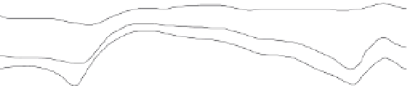
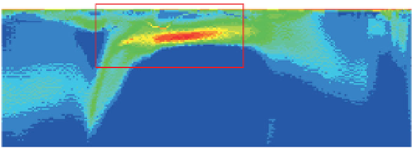
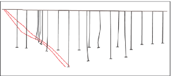
Figure 5.83
GEOTEM (75 Hz) airborne EM data from across
the Lisheen carbonate-hosted base-metal deposit. (a) Profile
plots, (b) conductivity parasection (the red rectangle shows the
extent of part (c)), and (c) geology. Redrawn, with permission,
from Nabighian and Asten (
2002
).
0
250
Metres
Massive sulphide mineralisation
Black matrix breccia
Limestone
Limestone/dolostone
Calcarenite/oolite
Another common presentation of amplitude data,
when data from multiple traverses are available, is a raster
display of the gridded amplitudes of a selected channel
(for examples, see
Section 5.9.5.1
). Computed decay and
time constants can also be displayed in this way. Images
are interpreted in a qualitative manner as described in
anomalous amplitudes do not resemble the sources of the
observed variations. The interpretation of data in this form
is described in Profile analysis in
Section 5.7.5.3
.
A second form of amplitude plot is the secondary decay
measured at specific stations, which may be analysed to
determine power-law decay and exponential time constants
to identify specific conductors (see
Figs. 5.78
and
5.81
).


Search WWH ::

Custom Search