Geoscience Reference
In-Depth Information
Table 5.5
The time-constant conductor shape-size factor
for
some common body shapes. Body dimensions are in metres.
S
+
Body shape
S
0
Time
-
r
2
Sphere, radius r
+
Cylinder, radius r, axis parallel to primary field
1.71r
2
Good quality (high
t
)
Disc, thickness t, radius r
1.79tr
Moderate
Thin plate, thickness t, average dimension L
tL
0
Poor quality (low
t
)
Time
2D plate, thickness t, depth extent l
2tl
-
+
Step response
size and depth, and
is the time constant, the time taken
for the signal to decay to 1/e or 36.8% of its initial value
and has the same units as t, usually milliseconds. The time
constant
τ
Poor quality (low
t
)
0
Time
Good quality (high
t
)
Moderate
has the same value for both the step and
impulse responses and depends on the conductivity and
the effective cross-section of the conductor and is given by:
τ
Impulse response
-
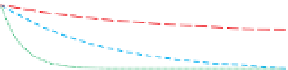
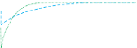
Figure 5.80
The exponential decays of a confined conductor of
poor, moderate and good quality schematically illustrated for the
step and impulse responses due to a perfect step turn-off of the
primary field. The reverse polarity of the impulse response is a
consequence of the negative sign in
Eq. (5.25)
. Redrawn, with
τ ¼
μσ
S
ð
5
:
26
Þ
π
2
where S is the shape-dependent size of the body (m
2
), for
which formulae for some common body shapes are given
in
Section 5.7.2.1
. Note from
Eq. (5.26)
that conductivity
τ
(large
) maintain the current system for a long time and
are referred to as late-time conductors. Poor conductors
(small
-
thickness product (see
Section 5.7.2.2
) is fundamental in
determining the response of plate-like conductors.
A graph of the logarithm of the signal amplitude on the
vertical axis versus the delay time on the linear horizontal
axis shows the exponential decay of
Eqs. (5.24)
and
(5.25)
as
a straight line with slope proportional to the inverse of
) lose the energy faster because of their higher
resistivity and are referred to as early-time conductors.
Note from
Eqs. (5.24)
and
(5.25)
, and as shown in
τ
0)
amplitude (A
0
) of the step response is the same for all values
of
¼
τ
(
Fig. 5.78b
). The shape of the conductor can be ascertained
from the spatial variation of the response across the survey
area, and its conductivity, for the appropriate model shape,
can be estimated using
Eq. (5.27)
(by rearranging
Eq. (5.26)
):
, i.e. it is independent of conductivity and depends on
the shape, size and depth of the body. For the impulse
response it is also inversely proportional to
τ
, i.e. it is mainly
inversely dependent on the quality of the conductor. So poor
conductors produce a high-amplitude eddy current
τ
ow at
first, but the energy is quickly lost. Good conductors pro-
duce a weaker eddy current at
first but maintain the current
system for a longer time. For both responses, measurements
to later times allow discrimination between good and poor-
quality conductors.
τ
σ ¼
ð
5
:
27
Þ
1
:
27
10
7
S
Conductor quality
The time constant
of the con-
ductor; a low value is indicative of a poor conductor having
low conductivity and/or small size, a high value indicative
of a good conductor having high conductivity and/or large
size. The value of
τ
quanti
es the
'
quality
'
Late-time measurements
When a conductive overburden layer is present and/or the
host/country rocks are conductive, their strong and fast
decaying power-law responses dominate at early to mid-
times (
Fig. 5.79
) and obliterate the weaker exponential
decays of confined conductors. In these situations the
confined conductor response will only be detectable at
τ
for mineralisation ranges typically from
μ
about 200
s to hundreds of milliseconds, and to several
seconds for very high-quality conductors; see for example
The time constant
and the conductor geometry control
the amplitude of the secondary field. Good conductors
τ


Search WWH ::

Custom Search