Electrical and electromagnetic methods - Geophysics for the Mineral Exploration Geoscientist - page 300

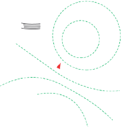
Figure 5.68 is a schematic representation of the EM
method. A time-varying electric current is passed through
the transmitter (Tx) to produce the primary magnetic field.
In accordance with Faraday

Continuously
varying primary
field

a)

s Law ( Eq. (5.7) ), when the
time-varying magnetic field intersects electrically conduct-
ive material eddy currents are induced within it. The eddy
currents have a magnetic field associated with them, the
secondary magnetic field, which is detected by the receiver
(Rx). Properties of the secondary field provide information
about the conductor.
We initially describe the EM method in general terms of
the two fundamental categories of EM measurements: fre-
quency domain and time domain measurements. This is
followed by descriptions of creating the primary field, the
induction and behaviour of induced eddy currents and,

'

Tx Rx

Conductor

finally, the detection and characterisation of the resulting
secondary magnetic field. Based on these fundamental

concepts, aspects of EM surveying are then described:
speci cally, the system geometry and system signal. System
geometry refers to the types of transmitter and receiver
used and the relative positions and orientations of their
antennae. System signal is the nature of the time variations
in the primary field and the way the secondary field is
characterised. These parameters determine the effective-
ness of the EM system in detecting particular discrete
conductors, mapping variations in a wide range of con-
ductivity and resolving shallow and deep targets.

Static
primary field

b)

I

Tx Rx

Conductor

5.7.1.1 Time domain and frequency domain EM
Electromagnetic systems vary the primary magnetic field
with time in one of two ways, as described in Section
5.2.2.2 , which leads to two classes of EM systems: time
domain (TDEM) and frequency domain (FDEM) systems.
In the time domain the change in the primary magnetic

c)

Tx Rx

field is produced by either abruptly turning off or turning
on a steady (d.c.) current. A pulse of current is induced in a
conductor. The eddy currents circulate in the conductor
for a short period and quickly decay as they lose energy.

Figure 5.68 Schematic illustration of an EM system used for
geophysical investigations. (a) The frequency domain case of a
continuously varying primary field. The diagram shows the situation

for a primary field increasing in strength, so the secondary field has
the opposite direction to oppose the change. (b) The time domain
case with a steady-state primary field shown before turn-off. (c)
Induced eddy currents and their secondary field following turn-off.
To oppose the change when the primary field is turned off, the
secondary field (broken lines) is detected by the receiver (Rx), which
is either a coil, shown here, or a magnetic sensor. Adapted from
Grant and West ( 1965 ).

Conductor

Primary
magnetic
field

Secondary
magnetic
field

Eddy
currents