Geoscience Reference
In-Depth Information
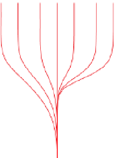
This is simply due to more of the current
flow taking the
path-of-least-resistance, preferring to
flow in the lower-
resistivity upper layer. When the resistivities are kept con-
stant and the thickness of the upper layer varied, the curve
behaves as would be expected and the change in apparent
resistivity occurs at increasingly larger X
AB
/2 as depth
increases (
Fig. 5.43b
)
.
Responses from three (or more) layers can be thought of
The component two-layer responses, affected by the rela-
tive resistivities and interface depths, combine to produce a
sounding curve that less resembles the resistivities, and, in
particular, the thicknesses of the various layers.
Figure 5.45
shows sounding curves for the six (A
a)
Apparent resistivity ( m)
1
0
0
10
1
10
2
10
3
10
0
Resistivity of upper layer
5
10
25
50
100
250
500
Upper
layer
10
1
20
10
2
Lower
layer
50
m
10
3
10
4
F) possible combin-
ations of three-layer relative resistivities. The true resistiv-
ities of both the upper and lower layers can be fairly
accurately determined from the soundings but information
about the middle layer is elusive. In particular, when the
resistivity of the middle layer is intermediate between those
of the upper and lower layers (models E and F) the
response is effectively identical to the two-layer case, so
the middle layer can be transparent unless it is particularly
thick. This is an illustration of a limitation of electrical
soundings; they are ambiguous (see
Section 2.11.4
)
. Put
simply, the same set of observations may be created by
signi
cantly different electrical layering, with obvious con-
sequences for interpretations.
There is an extensive literature on the interpretation of
electrical soundings, and forward and inverse modelling
software are widely available. These are usually based on a
1D model (see One-dimensional model in
Section 2.11.1.3
)
which assumes that the electrical structure of the ground is
a series of horizontal layers of constant resistivity and
chargeability and constant thickness. Many algorithms
attempt to account for ambiguity in the interpretation by
producing a range of possible solutions.
Departure from a 1D electrical structure is a serious
problem for electrical soundings. This is likely to occur at
larger array dimensions because the assumption of homo-
geneous horizontal layers often breaks down in the larger
volume of ground energised by the array. Lateral variations
in electrical properties and topography cause spurious
in
ections in the sounding curve, which can be mistaken
for layering (Pous et al.,
1996
).
A common application of electrical soundings in min-
eral exploration is investigation of the overburden, espe-
cially its thickness and internal variation in electrical
properties, often to facilitate an understanding or,
-
True resistivity of
lower layer (50 m)
b)
True resistivity of
upper layer (250 m)
Apparent resistivity ( m)
1
0
1
10
2
10
3
10
0
250
m
250
m
250
m
5
Upper
layer
250
m
10
1
10
5
10
25
50
25
50
10
2
Thickness of
upper layer
50
m
50
m
50
m
50
m
Lower
layer
10
3
10
4
True resistivity of
lower layer (50 m)
Figure 5.43
Computed Schlumberger array VES resistivity curves.
The curves are computed for a two-layer ground showing the change
in response for (a) a range of upper layer resistivity with constant
thickness, and (b) a range of upper layer thickness with constant
resistivity.
case half the current dipole length (X
AB
/2). The measured
resistivity at small electrode separations approaches that of
the upper layer, because then the current is chie
y con-
fined to the top layer. As the array expands the in
uence of
underlying layers on the measurements increases, so that at
larger separations the measured resistivity approaches that
of the lower layer. Clearly then, it is easy to identify the
relative resistivities of the two layers in the sounding curve,
but the depth to the interface between them is another
matter. Notice how the change in the curve occurs at
increasingly greater pseudo-depths as the upper layer
resistivity falls below that of the lower layer (
Fig. 5.43a
)
.
if


Search WWH ::

Custom Search