Geoscience Reference
In-Depth Information
Measurement of the decaying secondary voltage consists
of a number of discrete voltage measurements at selected
decay times. Usually the measurements are an average
taken over very small time-intervals, or channels, so they
approximately represent the area under the decay curve for
each measurement channel. Amplitude of the secondary
voltage is dependent upon the amplitude of the primary
voltage which depends on, apart from the subsurface resist-
ivity, the transmitted current. To account for this, the decay
voltage for each channel is normalised (divided) by the
primary voltage. This is known as the chargeability (M); it
has dimensions of time and is usually quoted in millisec-
onds. The value of M depends on the measurement period
and also on the width of the transmitted pulse, increasing as
either parameter increases. Values of M for all the decay
channels represent
Time
a)
Current (
I
)
On
On
+
Off
Off
Off
Off
0
-
On
Potential (
V
)
+
V
S
V
P
V
S
0
-
the polarisation decay. The entire
M
1
M
M
2
polarisation
decay cycle is repeated a number of times so
that the primary and secondary voltages can be stacked, or
averaged (see
Section 2.7.4.1
)
, by the receiver, after correct-
ing for the changing polarity of the current, to improve the
signal-to-noise ratio of the measurements. Modern instru-
ments can measure the secondary decay over a large
number of channels to provide an accurate de
nition of
can be adjusted which can make it dif
cult to directly
compare actual measurements from different surveys.
As for resistivity measurements (see
Section 5.6.2.1
), the
measured quantity corresponds to the true chargeability of
the ground only when the subsurface is electrically homo-
geneous; otherwise it is the apparent chargeability. A slow
or long decay is indicative of highly polarisable material, so
anomalously large chargeability at late decay times is con-
sidered significant.
-
M
3
t
1
t
2
t
1
t
2
t
3
t
4
t
5
t
6
Channels
Channels
b)
Higher
frequency
Lower
frequency
Curren
t
(
I
)
Current (
I
)
+
+
0
0
Potential (
V
)
Potential (
V
)
Lower-frequency
voltage (
V
Low
)
Higher-frequency
voltage (
V
High
)
+
+
0
0
c)
Current (
I
)
+
0
5.6.3.2
Frequency domain measurements
In the frequency domain, a.c. currents of different frequen-
cies are transmitted and the change in apparent resistivity
between each frequency is used as a measure of electrical
polarisation. In its most sophisticated form, frequencies
extending across the spectrum from 0.01 Hz to 1000 Hz
are used. This is known as spectral IP (SIP) (Wynn and
complex resistivity. The method has been successful in
Phase
shift
-
f
Potential (
V
)
+
0
-
Time
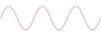
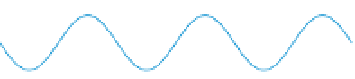
Figure 5.37
Signal waveforms used in resistivity and IP
measurements. (a) The time domain bipolar square wave signal and
the distorted wave measured by the receiver. Polarisation effects
produce the slow rise and decay in the received signal. The time
intervals used to measure apparent chargeability (M) are shown
shaded. (b) The frequency domain dual-frequency square wave
signals and the distorted waves measured by the receiver. (c) The
frequency domain sine wave signal and the phase-shifted wave
measured by the receiver.


Search WWH ::

Custom Search