Geoscience Reference
In-Depth Information
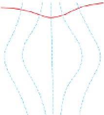
Conductive body
Resistive body
x
BM
a)
Stream line/current flow line
Current
electrode
Potential
electrode
V
I
To
To
A
N
B
M
Current flow
line
Equipotential
surface
Perspective
x
BM
Equipotential surface
Current
elect
r
ode
Potential
electrode
I
Permeable body
Impermeable body
V
To
To
A
B
M
N
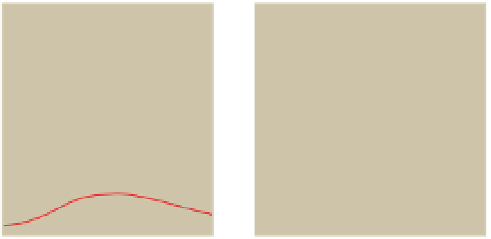
Figure 5.35
Distortions of the equipotential surfaces and associated
hydraulic/electric current flows due to zones that are more
permeable/conductive and less permeable/conductive than the
background material. Note that the current flow lines are
everywhere perpendicular to the equipotential surfaces.
Equipotential
surface
Current flow line
Cross-section
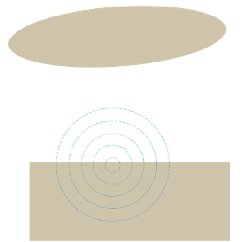
Consider the theoretical situation of an isolated current
electrode on the surface of an electrical half-space produ-
cing a hemispherical
b)
I
field in the subsurface (
Fig. 5.36a
).
The potential (V) is measured at a point located a distance
X from the current electrode, and with respect to zero
potential located at in
nity. The distance X is equivalent
to the length of the cylinder in
Eq. (5.3)
and the surface
area of the hemisphere (2
x
AN
x
BN
x
AM
x
BM
V
A
M
N
B
X
2
) is equivalent to the cross-
sectional area of the cylinder. Rearranging
Eq. (5.6)
gives
the resistivity of a substance as:
π
Figure 5.36
Current and potential electrodes. (a) Measurement of the
potential about an isolated current electrode on the surface and its
electric field in the subsurface. (b) The general configuration of
in-line electrodes used for measuring the resistivity of the subsurface.
V
I
k
geom
ρ ¼
ð
5
:
12
Þ
'
'
'
'
and the potential electrodes as
. Survey param-
eters can then be defined in terms of the distances between
electrodes, designated X
AB
and X
MN
. The potential at any
point is the sum of the potentials due to the two current
electrodes, which have opposite polarities (signs). The
resultant potential difference (
M
and
N
and applying
Eq. (5.3)
gives:
¼
X
2
X
V
I
2
π
V
I
ρ ¼
ð
2
π
X
Þ
ð
5
:
13
Þ
so for an electrode on the surface of a half-space
V) between the potential
electrodes due to each current electrode can be obtained by
applying
Eq. (5.15)
for each electrode and is given by:
Δ
k
geom
¼
2
π
X
ð
5
:
14
Þ
2
I
1
X
AM
1
X
BM
1
X
AN
+
1
X
BN
Δ
V
¼
ð
5
:
16
Þ
Rearranging
Eq. (5.13)
gives the potential at any point a
distance X from the electrode as:
π
Resistivity is obtained by rearranging
Eq. (5.16)
as follows:
I
ρ
I
ρ
1
X
1
V
¼
X
¼
ð
5
:
15
Þ
2
πΔ
V
1
X
AM
1
X
BM
1
X
AN
+
1
X
BN
2
π
2
π
ρ ¼
ð
5
:
17
Þ
I
Now consider the simplest situation for the resistivity
method: a half-space with both current electrodes and both
potential electrodes located anywhere on the surface
(
Fig. 5.36b
). When describing electrode arrays, convention
has it that the current electrodes are labelled as
Equation (5.17)
gives the true resistivity of an electrically
homogenous subsurface. That part of it representing the
effects of the electrode separations is the geometric factor
given by:
'
A
'
and
'
B
'


Search WWH ::

Custom Search