Geoscience Reference
In-Depth Information
For magnetic modelling, there is the additional compli-
cation of
a)
Bouguer
gravity (gu)
s magnetism (see
Sections 3.2.4
and
3.10.1.2
), which can be traded off against
changes in its geometry, usually its dip. Different combin-
ations of source dip and magnetism direction can produce
identical magnetic responses; this type of ambiguity is
illustrated in
Fig. 2.49c
. Failure to recognise the presence
of remanent magnetism which is not parallel
the direction of
the body
'
0
10
Kilometres
-400
-500
-600
-700
-800
to the
Location
b)
present-day Earth
s field will cause the model to be in
error, since the assumption of only induced magnetism
implies the source
'
0.0
s
field. Even when there is no significant remanent magnet-
ism, problems may occur owing to anisotropy of magnetic
susceptibility (see
Section 3.2.3.7
)
and, for the case of
highly magnetic sources, self-demagnetisation (see
Section
'
s magnetism to be parallel to the Earth
'
2.0
4.0
Maximum thickness
0.0
2.0
ect the induced
field away from parallel-
Minimum thickness
ism with the Earth
field.
The strategies described in
Section 2.11.4.1
, of using
knowledge of the nature of non-uniqueness to guide the
interpretation, can be applied in the analysis of gravity and
magnetic data. Of course, some prior knowledge of the
geology, and the target, is required in order to identify
realistic source geometries. Ideally there is also petrophy-
sical data available, but physical properties and especially
magnetic properties can vary by large amounts over small
distances (
Fig. 3.61
), so identifying the correct suscepti-
bility etc. to use can be equivocal. For these reasons, the
interpreter should create several models designed to repre-
sent
'
s
0.0
2.0
Most likely
Upper Bonnet Plume Fm (1.76 g/cm
3
)
Lower Bonnet Plume Fm & older Phanerozoic strata (2.55 g/cm
3
)
Basement (2.75 g/cm
3
)
Faults
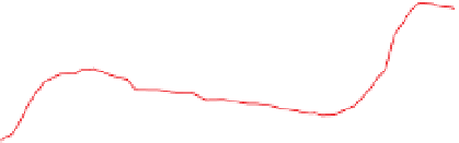
Figure 3.69
Model ambiguity in gravity data from the Bonnet Plume
Basin. (a) Observed gravity pro
le, and (b) cross-sections comprising
end-member density models: maximum and minimum thicknesses,
and what is considered to be the most likely model. Redrawn, with
permission, from Sobczak and Long (
1980
).
models of the range of possibilities: for
example the deepest possible source, the shallowest pos-
sible source etc. In practice, time constraints often mean
only one
'
end-member
'
interpretation is produced.
Figure 3.69
shows three gravity models across the
Bonnet Plume Basin, Yukon Territory, Canada. All are
geologically plausible and their responses (not shown)
'
preferred
'
types of mineral deposits, as would be sought during
exploration targeting, and to demonstrate various aspects
of their interpretation. Included are aeromagnetic data
from an Archaean granitoid
t
the data to an acceptable degree. The particular problem
was to determine the extent and thickness of the coal-
bearing upper and lower members of the Bonnet Plume
Formation. The models represent the maximum and min-
imum possible formation thickness, and also what is con-
sidered to be the mostly likely form of the underlying
geology.
greenstone terrain and
a low-grade metamorphosed Palaeozoic orogenic belt to
show the responses typical of these environments, and
to demonstrate the integrated use of potential
field data
for regional mapping, i.e. lithotype identi
cation, struc-
tural mapping and target identi
cation.
-
3.11.1
Regional removal and gravity mapping
of palaeochannels hosting placer gold
3.11
Examples of gravity and magnetic
data from mineralised terrains
This case study demonstrates the use of gravity to map
prospective stratigraphy, which in this case is low-density
palaeochannel
fill containing placer gold deposits. It illus-
trates the importance of regional gradient removal for
We present here a selection of examples to show the types
of gravity and magnetic responses produced by various


Search WWH ::

Custom Search