Geoscience Reference
In-Depth Information
a)
b)
Iron formation
n
= 195
Haematitic iron ore
n
= 150
n
= 48
2
0
m
10
-5
10
-3
10
-1
10
1
10
-5
10
-3
10
-1
10
1
Susceptibility (SI)
Susceptibility (SI)
Gneiss
n
= 405
Serpentinite
n
= 128
10
-4
10
-3
10
-2
10
-1
10
-4
10
-3
10
-2
10
-1
10
0
Susceptibility (SI)
Susceptibility (SI)
10
-5
10
-3
10
-1
10
1
10
-5
10
-3
10
-1
10
1
Susceptibility (SI)
Susceptibility (SI)
Figure 3.61
Magnetic susceptibility data from a thick komatiite
ow
in a greenstone belt in Western Australia. Measurements plotted (a)
in their locations across the
Amphibolite
n
= 126
Amphibolite
n
= 52
flow and (b) as a histogram. Based on
10
-5
10
-3
10
-1
10
1
10
-5
10
-3
10
-1
10
1
Susceptibility (SI)
Susceptibility (SI)
magnetic minerals within the dataset. A single-mode dis-
tribution is comparatively rare, even when the lithology
sampled appears homogenous.
Figure 3.61
shows suscepti-
bility variations through a thick komatiite
Gabbro
n
= 74
Basalt
n
= 159
flow. The zoning
of these
flows produces a complicated frequency histo-
gram, but the actual variation through the
flow is revealed
when the data are displayed in terms of their location
within the
ow.
It may be possible to distinguish both ferrimagnetic and
paramagnetic populations in the data. For this to occur in
fresh rocks the minerals of the two types must be segre-
gated within the rock at a scale greater than the dimensions
of the volume sampled by each measurement. In outcrop,
however, localised weathering may have oxidised titano-
magnetites to less magnetic species resulting in a measure-
ment influenced mainly by the paramagnetic constituents
of the rock. Statistical methods can be applied to suscepti-
bility data to identify individual populations; for example
Before applying statistical methods to a susceptibility
dataset, it is worth considering the purpose for which the
data were acquired. When the primary objective is to
delineate contrasts in magnetisation and to characterise
the magnetic responses of the various geological units,
a qualitative assessment of a complex distribution of sus-
ceptibility identifying a range of magnetic responses is
probably suf
cient. For example, the average or range of
susceptibility from a unit could be used to establish an
informal magnetisation hierarchy from
10
-5
10
-3
10
-1
10
1
10
-5
10
-3
10
-1
10
1
Susceptibility (SI)
Susceptibility (SI)
Diorite
n
= 251
Graphitic schist
n
= 35
10
-5
10
-3
10
-1
10
1
10
-5
10
-3
10
-1
10
1
Susceptibility (SI)
Susceptibility (SI)
Granite
n
= 337
Quartzite
n
= 20
10
-5
10
-3
10
-1
10
1
10
-5
10
-3
10
-1
10
1
Susceptibility (SI)
Susceptibility (SI)
Red sandstone
n
= 60
Kimberlite
n
= 375
10
-5
10
-3
10
-1
10
1
10
-5
10
-3
10
-1
10
1
Susceptibility (SI)
Susceptibility (SI)
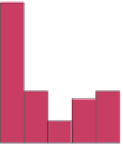
Figure 3.60
Frequency histograms of magnetic susceptibilities for
various lithotypes. The data for each lithotype are from the same area
and are all measurements made on outcrop. Based on diagrams in
of the authors. Note how bi-modal or multi-modal successions
are the norm.
'
highly magnetic
'
'
'
but not invariably, the distribution will be skewed, so it is
usual to plot the logarithm of susceptibility to make the
frequency distribution more symmetrical (Irving et al.,
1966
)
. The data are often multimodal (
Figs. 3.47
and
3.60
) owing to the presence of different populations of
through to
and to which the likely geology
in concealed areas could be referred. Although statistical
analysis may be unnecessary for these applications,
adequate sampling to create a representative distribution
is essential.
non-magnetic


Search WWH ::

Custom Search