Gravity and magnetic methods - Geophysics for the Mineral Exploration Geoscientist - page 121

c)

a) b)

2
Kilometres

0

Las Cruces

d) e) f)

g) h)

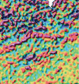
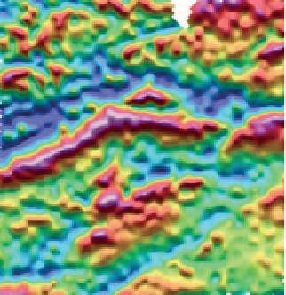
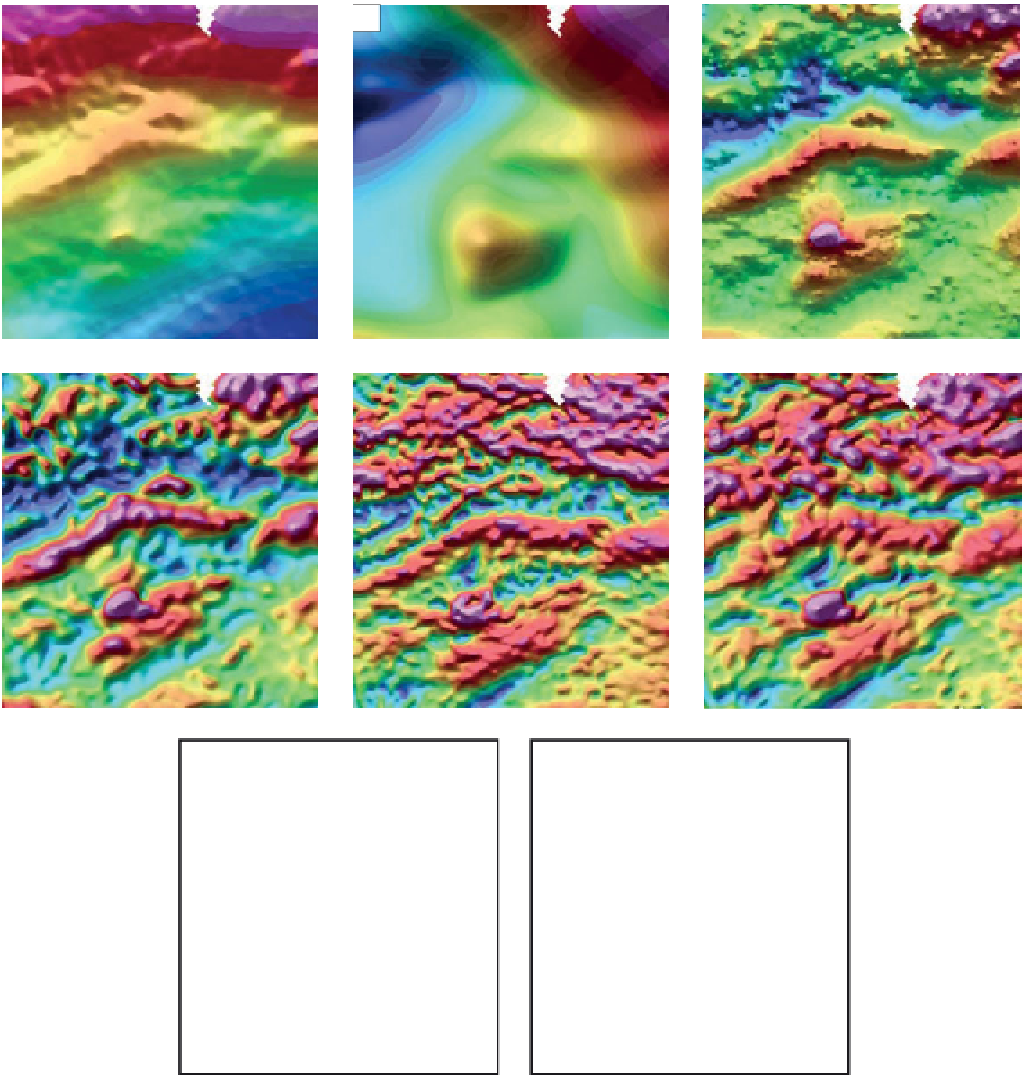
Figure 3.27 Gravity data from the vicinity of the Las Cruces Cu

Au massive sulphide deposit. All images are pseudocolour combined with
grey-scale shaded relief illuminated from the northeast. (a) Bouguer gravity, (b) data in (a) upward-continued by 800 m, (c) residual dataset
obtained by subtracting (b) from (a), (d)

-

rst t vertical derivative, (e) total horizontal gradient of data in (a), (f) 3D analytic signal of data in (a),
(g) tilt-derivative of data in (a), and (h) second vertical derivative of data in (a). The arrows highlight a prominent linear feature. Note
how this is more easily seen in the various derivative-based enhancements.

Caption for Figure 3.26 (cont.) (d) TMI reduced-to-pole data: note the symmetrical response, revealing the form of the source, unlike the
complex TMI anomalies in (a). (e) First vertical derivative of reduced-to-pole data in (d): note the symmetrical response revealing the form of
the source more clearly than the complex derivative anomalies in (b). (f) Pseudogravity response; compare with Fig. 3.25a . (g) Total horizontal
gradient of pseudogravity response in (f), again revealing the form of the source. (h) Tilt-derivative of reduced-to-pole data in (d). Note the
positive response of the source. The responses in (c) to (h) are more easily correlated with the source geometry than the non-polar responses in
(a) and (b).