Geoscience Reference
In-Depth Information
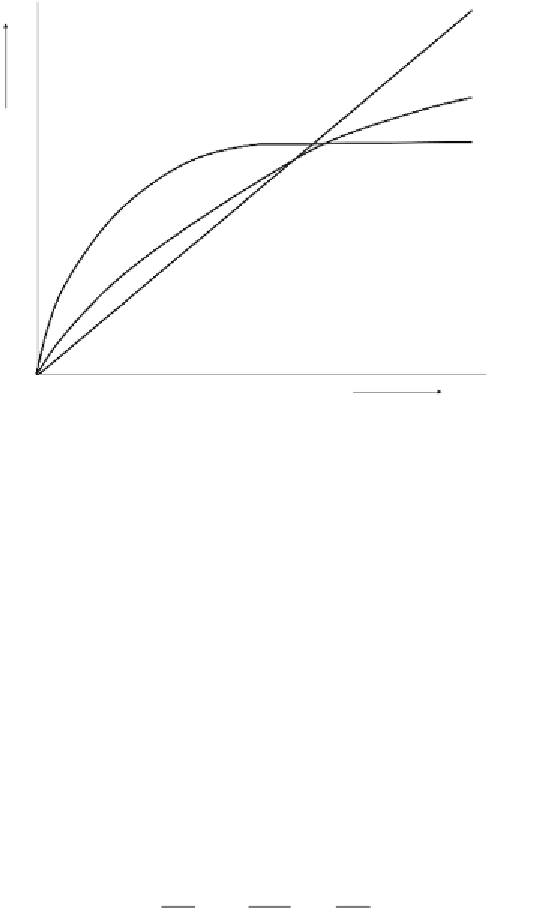
Linear:
C
a
=
S
d
C
I
Freundlich:
1/N
C
a
=
K
f
C
I
aTC
I
1 +
aC
I
Langmuir:
C
a
=
Dissolved concentration
C
l
Figure 5.7
Three main adsorption isotherm shapes with their analytical expression.
dissolved and adsorbed phases are instantaneously in equilibrium), then the time
derivative of
C
a
may be written as:
∂
∂
=
C
t
∂
∂
C
t
a
S
l
(5.15)
d
Using Eq. (
5.15
), Eq. (
5.13
) can be written as:
2
ρ
θ
S
∂
∂
=
C
t
∂
∂
C
z
−
∂
∂
=
∂
C
z
C
t
1
+
bd
l
D
l
v
l
R
l
(5.16)
e
2
∂
bd
/
(-) is deined as the
retardation factor
. The retardation fac-
tor equals the total solute amount in a soil volume divided by the dissolved solute
amount. Finally, we may divide each side of Eq. (
5.16
) by
R
, producing:
where
R
=1
ρθ
S
2
∂
∂
=
C
t
∂
∂
C
z
∂
∂
C
z
l
D
l
−
v
l
(5.17)
R
R
2
where
D
R
=
D
e
/ R
and
v
R
=
v / R
are the retarded dispersion coeficient and solute
velocity, respectively.
Let us add adsorption to the column leaching experiment of
Figure 5.2
.
Figure 5.8
shows the effect of adsorption without considering dispersion. In the case of
R
= 2,
the solutes move at a velocity
v
/2 cm d
-1
. Note that the surface of the area below the
curve is 50% of the area in case of
R
= 1 (no adsorption) because at
R
= 2 only 50% of
the solutes are in the soil water solution.
Figure 5.9
includes the effect of dispersion.


Search WWH ::

Custom Search