Geoscience Reference
In-Depth Information
1.00
0.90
0.80
0.70
0.60
0.50
0.40
0.30
L
dis
= 0 cm
L
dis
= 10 cm
0.20
0.10
0.00
20
40
60
80
0
100
Time (d)
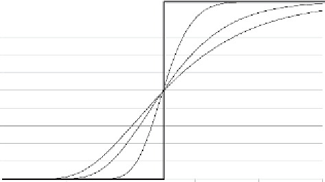
Figure 5.5
Breakthrough curves for the experimental data listed in
Figure 5.2
and for
different values of dispersion length (
L
dis
= 0, 1, 5 and 10 cm).
and the average annual recharge rate
q
= 0.25 m y
-1
. The residence time
T
res
can be
calculated as:
L
v
θ
015 0
025
L
q
.
×
T
== =
=
6
years
(5.11)
res
.
Question 5.7:
In the Netherlands the recharge of the groundwater amounts to ca.
250 mm y
-1
. Determine the residence time of inert, nonadsorbing solutes in the unsatu-
rated zone in case of the Veenkampen (peat soil,
θ
= 0.64,
L
= 0.5 m) and Otterlo (sand
soil,
θ
= 0.14,
L
= 20.0 m).
Often a narrow solute pulse, rather than a front, might be added to a soil.
Figure 5.6
shows for the soil column of
Figure 5.2
the corresponding outlow curves for a narrow
pulse input
C
0
= C(0,
t
) Δ
t
(kg d m
-3
) in which Δ
t
is the relatively short application
time. The mathematical solution to Eq. (
5.9
) for a solute pulse added to a clean soil
is (Jury and Sposito,
1985
):
−
−
( )
2
z t
Dt
()
=
−
zC
Dt
Czt
0
exp
(5.12)
4
2
π
e
3
e
A pulse of 1 day was applied with the concentration
C
(0,
t
) = 1000 μg L
-1
. As
Figure 5.6
shows, the maximum concentration decreases rapidly due to dispersion. Note also
that the curves are asymmetric, because as time increases, dispersion causes a larger
spreading (Jury et al.,
1991
).


Search WWH ::

Custom Search