Geoscience Reference
In-Depth Information
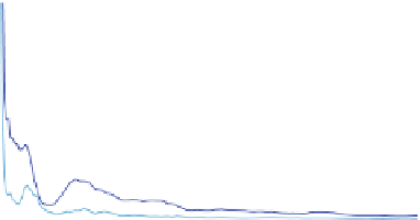
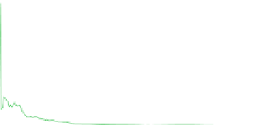
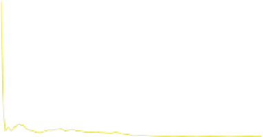
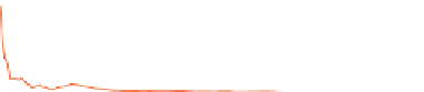
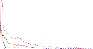
Fig. 3.3
Plots of the
R-statistic for successively
greater numbers of samples
(see text for derivation and
explanation) for each of ten
estimated parameters
1.5
1.4
1.3
1.2
1.1
1.0
0
5 10
Number of Samples (x1000)
15
20
The between-chain variances are computed as
X
m
x
j
x
2
n
m
1
B
D
;
(3.12)
j
D
1
where
x
is the mean of the given parameter across all chains
X
x
D
1
m
x
j
:
(3.13)
j
D
1
x
An unbiased estimate of the marginal posterior variance of each parameter
condi-
tioned on the set of observations
y
can be obtained from a weighted combination of
B
W
and
as
b
/
D
n
1
n
W
C
1
ar
C
.x
j
y
v
n
B:
(3.14)
This quantity tends to overestimate the true marginal posterior variance, but
converges to the true variance as
n
!1. Proper chain mixing is assessed by
comparing the variance estimate to the within-chain variance, and computing the
R-statistic
,
R;
an estimate of the factor by which the dispersion in the current sample
would be reduced if each chain were allowed an infinite length
r
var
C
.x
j
y
c
/
R
D
:
(3.15)
W
It can be readily seen from (
3.14
) that this estimate will converge to 1 in the
limit as
n
!1. According to
Gelman et al.
(
2004
), there is no specific value
of the r-statistic for which chains can be said to have sufficiently mixed, though a
value of
R
less than 1.1 for each parameter is generally deemed acceptable. An
illustration of convergence of within and between-chain variance for increasing
numbers of samples for an 8-chain MCMC experiment is depicted in Fig.
3.3
.It
can be seen that by approximately 5,000 iterations, the chains can be assumed to
have mixed sufficiently as their
R
value drops below 1.1, and between 5,000 and
R
10,000 iterations
drops below 1.05 and levels off.


Search WWH ::

Custom Search