Geoscience Reference
In-Depth Information
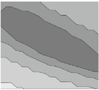
Fig. 10.2
The maximum
time before linearity breaks
down for the “regular” regime
using perturbations in
14
1.5
12
1
x
or
y
of varying sizes
10
0.5
8
0
6
−0.5
4
−1
2
−1.5
0
−1.5
−1
−0.5
0
0.5
1
1.5
δ
x
equal to the initial error are too great to be considered weakly nonlinear; however,
these time window estimates provide an upper time bound for the experiments.
AsisshowninFigs.
10.1
and
10.2
, the prescribed initial error is significant to
determining the time window of the system. No matter the growth of the nonlineari-
ties, a longer period can be used with smaller initial error as the error growth rate can
be approximated by
P
2
e
t
.Ifthe
prior
error,
P
, is small, long time-windows are pos-
sible. Figure
10.1
b shows that despite the large growth of linear error, long window
solutions are possible if
P
is small. The linear and nonlinear cost functions deviate
illustrating that this system is not fully linear over the periods of interest, and it
provides an ideal configuration to examine the role of constraints in the outer-loops.
Ensembles of twin experiments are created to compare the two separate cost
functions. The regular and transition initial conditions were integrated for the
predetermined time window to generate truth trajectories then sampled to generate
the observations. Observations were equally spaced over the time window avoiding
the starting and ending times and each state variable was sampled an equal
number of times, such that at each observation time, the entire state is observed.
An ensemble of 500 members was created by randomly perturbing the initial
conditions with variance consistent with
P
. For each ensemble member, random
error consistent with
R
was added to each observation. Initially,
P
and
R
were
chosen as diagonal matrices with elements set to 2. Each member assimilated the
randomly perturbed observations using four outer-loops with both the overfit and
constrained data-space methods as well as with sequentially applied 3D-Var. The
3D-Var was applied at each time of the full state observations during the time
window of interest. After applying the 3D-Var, the system was integrated to the
next set of observations, and the 3D-Var is repeated with the same
P
and
R
and
using the current state as
x
b
. Unlike the 4D-Var solutions, the 3D-Var solutions
are discontinuous during each of the examined time windows and
posterior
statistics discussed below are not readily available. The time window was taken as


Search WWH ::

Custom Search