Geoscience Reference
In-Depth Information
1
0.8
0.8
0.6
0.6
0.4
0.4
0.2
0.2
0
0
−0.2
0
2
4
6
8
0
1
2
3
4
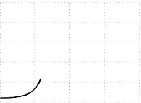
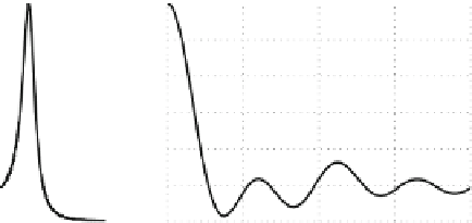
Fig. 8.3
An
example
of
the
normalized
spectrum
(
left
)
and
the
respective
correlation
function
(
right
)
for
the
fourth-order
polynomial
(
8.26
)
in
two
dimensions
(
M
D
2
I
z
1
D
:5
C
3i
I
z
2
D
:2
C
6i
)
In practical applications, a BEC model is often constructed by fitting the spectral
(
8.25
) or correlation (
8.28
) functions to those derived from experimental data.
These functions are characterized by
parameters which give enough freedom for
approximating complex spectra. The approximation procedure can be formulated as
a least squares problem in
2m
2m
dimensions, which may be rather difficult to solve due
to the non-linearity of
b
m
. Therefore,
it is useful to have guidance on how the BEC model parameters are related to the
scales and amplitudes of the physical modes that contribute to the experimental
spectrum (Fig.
8.3
).
The contribution of the
B
with respect to the fitting parameters
a
m
and
th mode to the spectrum can be assessed by integrating
the right hand side of (
8.26
):
m
q
m
k
2
C
z
2
m
Z
q
m
k
2
C
z
2
m
dk
D
h
q
m
z
m
i
j
z
m
j
2
E
m
D
C
(8.36)
0
In the limit when distances j
b
l
b
m
j between the spectral peaks of
B
are much larger
than their half-widths
a
m
,(i.e.
a
m
=b
m
0
in particular), (
8.36
) can be simplified
using the asymptotic approximations
4ia
m
˘
m
I
˘
m
Y
j
¤
m
b
m
.1
b
m
=b
j
/
2
z
m
ib
m
I
q
m
to yield
b
m
E
m
4a
m
˘
m
:
(8.37)
Asymptotic values of the spectral density at the peaks are respectively
b
m
4a
m
˘
m
D
E
m
B.b
m
/
a
m
;
(8.38)


Search WWH ::

Custom Search