Geoscience Reference
In-Depth Information
1
1
m=
m=
∞
m=3
m=2
m=1
∞
m=3 n=2
m=2 n=2
m=1 n=1
0.1
0.8
0.8
0.05
0
0.6
0.6
−0.05
0.4
0.4
−0.1
m=
∞
m=3 n=2
m=2 n=2
m=1 n=1
−0.15
0.2
0.2
−0.2
0
0
−0.25
0
1
2
3
0
2
4
0
2
4
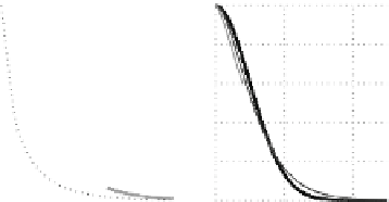
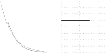
Fig. 8.1
Left
: Binomial approximations (
8.13
) of the Gaussian CF in two dimensions (
n
D
2
).
The CF for
m
D
1
is shown by the
dotted line
for the numerical realization with the grid step
ı
D
a=4
.
Middle
: Same approximations, but with optimally adjusted correlation radii for various
combinations of
.
Right
: Differences between the Gaussian CF and its approximations
shown in the
middle panel
.The
horizontal axes
are scaled by
m
and
n
a
are both positive and have similar shapes, a reasonable optimization criterion is to
set their integral decorrelation scales equal to each other:
p
Z
Z
Z
C
m
./dr
a
opt
.
r
2
a
p
C
m
.y/dy
D
p
exp
2a
2
/dr
D
2
:
(8.16)
2m
0
0
0
a
opt
D
m
a
m
Expression (
8.16
)showsthat
, where the rescaling coefficient
is
defined as:
2
3
1
Z
m
D
p
.s/
.s
C
1=2/
p
4
5
C
m
.y/dy
m
D
m:
(8.17)
0
m
for
The values of
m;n < 4
and their respective approximation errors
Z
Z
e
m
D
j
C
m
C
1
j
dr=Œ
j
C
1
j
dr
0
0
areassembledinTable
8.1
.
The coefficients
m
along with relationship (
8.12
) provide an expression for
estimating the scaling parameter in the binomial model (
8.10
) which approximates
the Gaussian-shaped CF with a given radius
a
:
p
D
m
a=
a
binom
2m
(8.18)


Search WWH ::

Custom Search