Skewness of the Prior Through Position Errors and Its Impact on Data Assimilation - Data Assimilation for Atmospheric, Oceanic and Hydrologic Applications - page 154

a b

1000 1000

995 995

990 990

985 985

980 980

975 975

975 980 985 990 995 1000 975 980 985 990 995 1000

p(x=0) p(x=0)

c d

1000 1000

995 995

990 990

985 985

980 980

975 975

975 980 985 990 995 1000 975 980 985 990 995 1000

p(x=0) p(x=0)

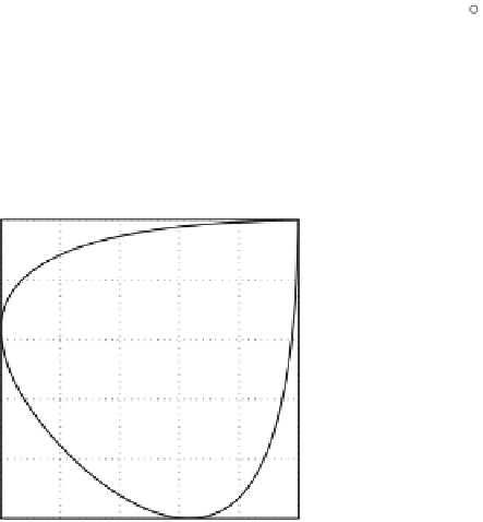
Fig. 7.2 The structure of phase error distribution as loops. In ( a ) is the distribution of pressure
between x D 0 and x D 1 ,( b )isforx D 0 and x D 1:4 ,( c )isforx D 0 and x D 2 ,and( d )isfor

x D 0 and x D 4 .The open circle in each panel denotes the location of the mean

The pattern found in Fig. 7.1 b is consistent with the analysis presented above in so
far as the third moment is positive at the center of the distribution and decreases
to zero near the inflection point. Figure 7.1 b reveals however that the third moment
actually turns negative outside of the inflection points leading to a tri-pole structure.
This tri-pole structure in the third moments depends on the strength of the phase
error variance of

'

. When the phase error variance is large, rendering the assump-
tions about truncating the Taylor-series invalid, the tri-pole pattern in the third
moments is replaced with a relatively wide monopole negative region (not shown).
To gain understanding of the multivariate structure we plot in Fig. 7.2 the
distribution of pressure values at the center of the distribution

.x D x 0 /

against
the values of pressure at various locations for the same Gaussian phase error