Mantle Mixing: Processes and Modeling - Physics and Chemistry of the Deep Earth - page 360

those seen in global tomographic models. We
can also directly compare the physical structure
of a model with that seen in tomography. For
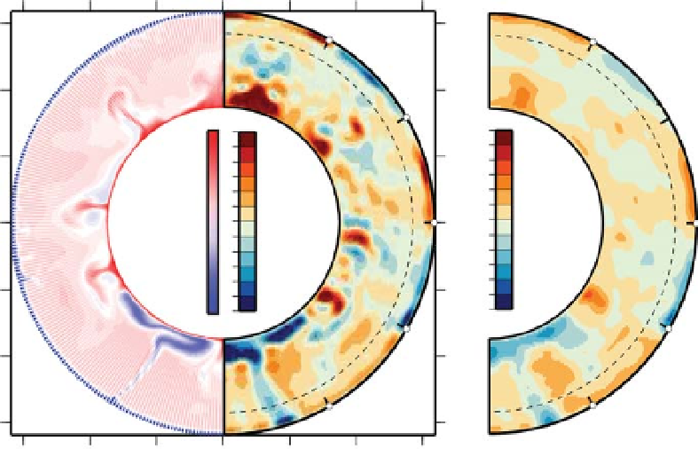
example, we take the model of Figure 12.1 and
convert this using self-consistent thermodynam-
ics (Cobden et al ., 2008) to the seismic velocity
perturbation that would be caused by the ef-
fects of temperature and composition (Figure 12.6,
middle frame). We can then use the resolution fil-
ters provided by the S40RTS tomographic model
(Ritsema et al., 2011) to see how the velocity
anomaly would be imaged in the seismic to-
mography (Figure 12.6, right frame). This is a
powerful technique, as it directly takes into ac-
count the variable resolution of the tomographic
model and allows us to estimate how a particular
velocity structure would be recovered in the to-
mographic model. A direct comparison between
this model-derived seismic ''image'' and a Pacific
cross-section through the S40RTS model suggest
some reasonable similarities. The size and height

extent of the large low shear-velocity province is
similar, and the amplitude and geometry of the
subducting slab in this model looks similar to
the imaged Farallon slab, which may suggest that
the relatively simple rheology employed in the
dynamical model suffices to recreate the shape
of subducting slabs in the present-day Earth. In-
terestingly, the image from the dynamical model
looks smoother than the tomographic model it-
self, and there is a stronger separation between
upper and lower mantle in the tomography than
in the Brandenburg model, suggesting that the
mantle may be more strongly layered than the
Brandenburg model.
In summary, we have modeled the evolution
of the Earth's mantle using the formation and
recycling of oceanic crust. For models that have
earthlike convective vigor, as measured by surface
heat flow and plate velocities, we find a reason-
able agreement in the isotopic evolution with
the observed data in multiple isotope systems.

6000

4000

− 5%

− 2.5%

3273 K

2000

0

2000

−

+ 2.5%

+ 5%

273 K

− 4000

− 6000

0 2000 4000 6000

− 6000 − 4000 − 2000

x (km)

(a) (b) (c)

Fig. 12.6 We map temperature (left) and eclogite fraction (not shown) into shear velocity variations using the
mineralogical conversions of Cobden et al ., 2008 (middle). The right frame shows the prediction how the shear
velocity variations would be recovered in S40RTS (Ritsema et al ., 2011). Reproduced with permission of John Wiley
& Sons. (See Color Plate 14).