Geoscience Reference
In-Depth Information
S40RTS at 100 km depth
S40RTS at 500 km depth
S40RTS at 2800 km depth
−
7.5
+
7.5
−
3.0
+
3.0
−
3.0
+
3.0
null-space component
at 100 km depth
null-space component
at 500 km depth
null-space component
at 2800 km depth
1.5
1.5
0.6
0.6
0.6
0.6
−
+
−
+
−
+
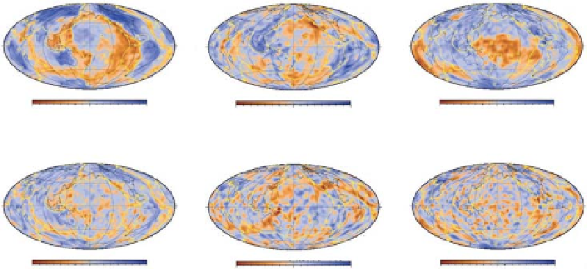
Fig. 11.1
Top Relative S velocity variations,
d
ln
v
s
, in the global model S40RTS (Ritsema
et al.
, 2011) at 100, 500
and 2800 km depth. Bottom: The corresponding null-space component
m
null
. The null-space component contains
short-wavelength structure that can be scaled and added to the model without changing the misfit. (See Color
Plate 11).
˜
With a few notable exceptions (e.g., Bijwaard
& Spakman, 2000; Panning & Romanowicz,
2006), all classical P- and S-velocity models are
obtained by a linear inversion using expression
(11.2). The most important tool to assess the
amplitude and shape of the models obtained by
linearized inversions is the resolution operator,
provided that the influence of the data errors is
small (Equation 11.3). The latter is the case for
most strongly regularized models. The resolution
is an operator which tells us how the obtained
model parameters are linearly related to each
other. Ideally we would like to construct a
model such that the resolution is the identity
matrix, meaning that the data can constrain
all the chosen parameters separately with the
correct amplitude. A typical global seismic
tomography model consists of few thousand to
a few hundred thousand model parameters, and
this number squared is the number of entries
in the resolution matrix. It is therefore easily
understandable that the latter can computation-
ally be a challenge, although not impossible
(e.g., Soldati
et al.
, 2006). The importance of
calculating the resolution matrix was put forward
for comparing seismic tomography to geodynamic
models (e.g, Ritsema
et al.
, 2007), but more often
than not simple synthetic tests of the chequer
board type are used as a proxy for the resolution
matrix. (Lev eque
et al.
1993) convincingly argued
that such a simple test has to be interpreted with
caution as it can be quite misleading and hardly
representative of the true resolution.
As a result of regularization, most resolution
tests indicate that only a quarter to a third of the
amplitude of heterogeneities is recovered (e.g., Li
et al.
, 2008; Ritsema
et al.
, 2007). This observa-
tion is crucial, but often forgotten, when combin-
ing seismic tomography and mineral physics data
to estimate the thermo-chemical structure of the
mantle. Equation-of-state modeling (e.g., Karato
& Karki, 2001; Trampert
et al.
, 2001; Stacey
& Davis, 2004; Stixrude & Lithgow-Bertelloni,
2005; 2011) of mineral physics data allows us
to infer sensitivities (partial derivatives) of ve-
locity variations to temperature and chemical
variations. To make the conversion, amplitude
and position of the seismic anomalies has to be
known with great precision. For instance, if only
temperature is changing at a depth of 2800 km,