Geoscience Reference
In-Depth Information
In these calculations, (1) the ionic positions
need to be reoptimized in the strained lattice
in order to incorporate any couplings between
strains and vibrational modes in the crystal (Nas-
tar & Willaime, 1995); (2) the elastic constants
need to be computed in the appropriate limit of
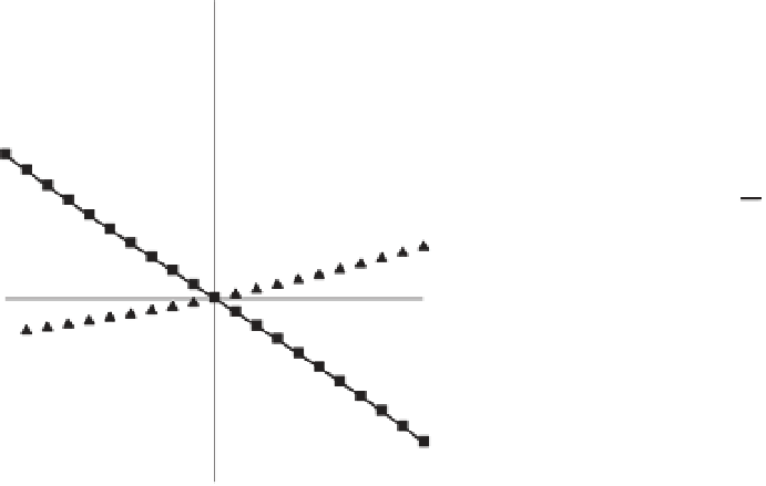
zero strain. At finite strain, higher-order terms in
the stress-strain relationship become important
(Figure 7.1). To calculate the elastic constants in
the linear regime, which is appropriate for the geo-
physical condition, strains of different magnitude
or sign are applied, and the zero-strain limit is
determined by interpolation. The elastic constant
tensor originally has 81 independent components,
while they are reduced to 21 by the commutative
symmetries with respect to (
i
,
j
), (
k
,
l
), and (
ij
,
kl
).
They are further reduced depending on the crys-
tal symmetry to 13, 9, 7, 6, 7, 6, 5, and 3 for
monoclinic, orthorhombic, tetragonal with 4,
4
,
4
/m
point group symmetry (PGS), tetragonal with
422, 4mm,
42
m
,4/
mmm
PGS, trigonal with 3,
3
PGS, trigonal with 32, 3m,
3
m
PGS, hexagonal,
and cubic, respectively. After obtaining the sin-
gle crystal elastic constant tensor, polycrystalline
isotropic elasticity, bulk and shear moduli, can be
calculated based on relevant averaging schemes.
Although the most appropriate method for averag-
ing is still unclear for the geophysical condition,
the most often applied one is the Voigt-Ruess-Hill
average (Hill, 1952) or Hashin-Shtrikman average
(Hashin-Shtrikman, 1962). The isotropic averaged
compressional (P), shear (S), and bulk (
)wave
velocities can be then calculated as
B
+
B
ρ
,
(7.6)
respectively. Combining this technique,
ab ini-
tio
lattice dynamics method (Baroni
et al
., 1987,
2001) and quasiharmonic approximation (Wal-
lace, 1972), the calculation condition was suc-
cessfully extended to finite temperature with
including phonon thermodynamics (Karki
et al
.,
1999; Wentzcovitch
et al
., 2004, 2006).
Calculations of finite temperature elastic con-
stants are considerably heavier than that of static
elasticity. There are two different techniques to
include thermal contributions: one is the lattice
dynamics method, and another is the molecu-
lar dynamics method. In the former approach,
one first calculates finite-temperature free energy
for strained conditions by applying the quasi-
harmonic approximation, determines isothermal
stiffness
c
ij
(
P
,
T
) based on the energy-strain rela-
tion (not on the stress-strain) as
G
ρ
,and
V
=
4
3
G
V
P
=
,
V
S
=
ρ
60
σ
1
40
∂
2
G
∂ε
ij
∂ε
kl
1
V
c
ijkl
=
,
(7.7)
20
σ
2
T
and then converts them to adiabatic quantities
c
ij
(
P
,
T
)(Karki
et al
., 1999; Wentzcovitch
et al
.,
2004, 2006). Lattice dynamics calculation must
be performed for each strained cell at each static
pressure, leading to huge data sets to be man-
aged. In contrast, in the latter approach,
c
ij
(
P
,
T
)
are determined based on the usual stress-strain
relation as the static calculations of elasticity,
but sufficiently long simulations with large su-
percells are required to get accurate averages of
the stress tensor, leading to significant computa-
tion time. Therefore, the size of supercell used
0
σ
4
−
20
−
40
−
0.10
−
0.05
0
+
0.05
+
0.10
Strain
Fig. 7.1
Stress-strain relations calculated for MgO at 0
GPa up to
ε
=±
0.1.