Geoscience Reference
In-Depth Information
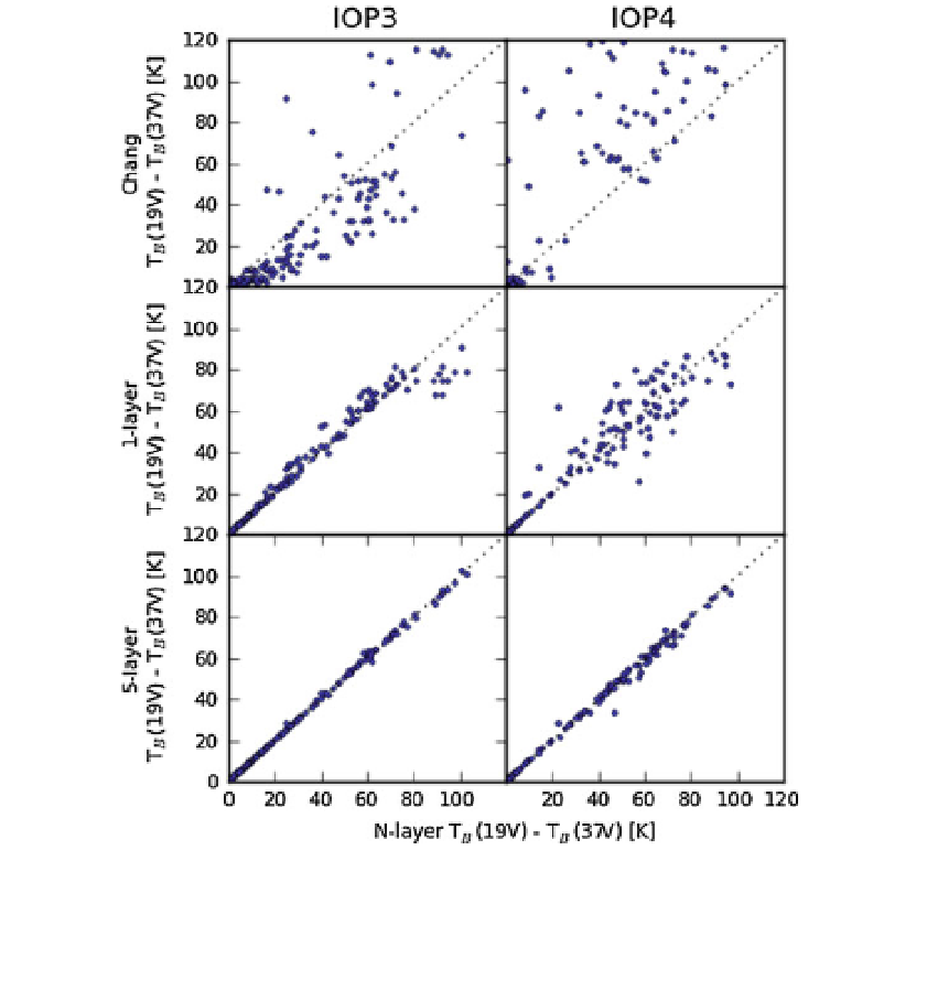
Fig. 7 Brightness temperature differences simulated for each pit during intensive observation period (IOP)
3(left) and IOP4 (right). The ordinate in each case is the simulated brightness temperature difference using
the N-layer model, and the abscissa shows the Chang output (top), 1-layer Helsinki University of
Technology model (HUT) output (centre) and 5-layer HUT (bottom) output as labelled. The dotted line is
the one-to-one correspondence line
from the single-layer model's brightness temperature sensitivity to grain size, and the
statistics of the ensemble of nearest station grain sizes.
It was suggested in Sect.
3.2.2
that future implementations of Globsnow might be
improved by using a LSM to provide grain size estimates in every grid cell, thus
accounting for regional changes in geography and meteorology that are beyond the
Globsnow kriging approach, and for the well-noted bias in observation location towards
low latitudes, altitudes and canopy cover.
Even if an LSM were to provide the snow state forecasts, the current weighting scheme
would not account for the variance introduced by its simplified layering relative to the
truth. The LSM could be allowed to increase in complexity and contain more layers, but
computational expense would rise both in the forecast step and in solving the update
equation as the snow state vector and relevant covariance matrices would grow to contain
more layer properties.
A user could apply the approach adopted here to estimate the extra variance introduced
to their simulations as a function of the snow depth and their layering structure. Taking the