Geoscience Reference
In-Depth Information
symbols:
u
u
u
. Over a longer time period, the mean
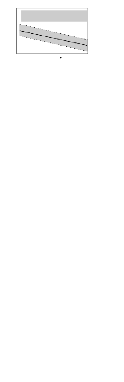
Steady flow in the mean
+u
rms
of
u
is positive and negative about
the mean at different times. The instantaneous magnitude
of
u
must be zero, since
u
Time mean
u
-u
rms
gives us a measure of the instantaneous magnitude of
the turbulence. But what about the longer-term magni-
tude; can we somehow characterize the fluctuating system?
Although the long-term value of
u
+u
rms
is zero, the positive
and negative values all canceling, there is a statistical trick,
due originally to Maxwell, that we can use to compute the
long-term value. If we square each successive instanta-
neous value over time, all the negative values become pos-
itive. The mean of these positive squares can then be
found, whose square root then g
ive
s what is known as the
root-mean-square fluctuation
,
Time mean
u
-u
rms
0
Time
Fig. 3.46
Turbulent flow velocity time series in
u
, the streamwise
velocity component.
(
u
2
)
0.5
or in shorthand,
u
rms
. This is how we express the mean
turbulent intensity
component of any turbulent flow. Similar expressions for
the vertical,
w
, and spanwise,
v
, velocity components give
us a measure of the
total turbulent intensity
,
q
Any instantaneous velocity comprises the time
mean velocity + the instantaneous fluctuation
+w'
rms
rms
(
u
rms
v
rms
w
rms
).
Steady flow in the mean
+w'
rms
3.11.3
Steady eddies: Carriers of turbulent friction
Time mean
w =
0
0
-w'
rms
Turbulent flows are very efficient at mixing fluid up
(Fig. 3.48) - far more so than simple molecular diffusivity
can achieve in laminar flow. Since mixing across and
between different fluid layers involves accelerations, new
forces are set up once turbulent motion begins. These are
-w'
rms
Fig. 3.47
Turbulent flow velocity time series in
w
, the vertical velocity
component.
3.11.2
Fluctuations about the mean
Quite what to do about the physics of turbulent flow
occupied the minds of some of the most original physicists
of the latter quarter of the nineteenthcentury. Reynolds'
finally solved the problem in 1895 using arguments for
solution of the equations of motion (Newton's Second
Law as applied to moving fluids; see Section 3.12). These
were partly gained from experiments (Section 4.5) into the
physical nature of such flows and from analogs with nas-
cent kinetic molecular theory of heat and conservation of
energy. The solution Reynolds' came up with was that
both the magnitude of the mean flow
and
of its fluctuation
must be considered: both contribute to the kinetic energy
of a turbulent flow. To illustrate this, take the simplest
case of steady 1D turbulent flow (Fig. 3.46); the arith-
metic gets quite cumbersome for 3D flows (see Cookie 8).
The instantaneous longitudinal
x
-component of veloci
ty
,
u
, is equal to the sum of the time-mean flow velocity, ,
and the instantaneous fluctuation from this mean,
u
Flow
Fig. 3.48
Turbulent air flow in a wind tunnel is visualized by smoke
generated upflow close to the lower boundary. The top view shows
the flow from above, the thin light streak along the central axis
being the intense beam of light used to simultaneously illuminate
the lower side view. Turbulent eddies are mixing lower speed fluid
(the smoky part) upward and at the same time transporting faster
fluid downward.
u
. In


Search WWH ::

Custom Search