Geoscience Reference
In-Depth Information
x 10
6
x 10
5
6
(a)
(b)
3
4
2
2
1
0
0
-1
-2
-2
-4
-3
-6
4
-3
-2
-1
0
1
2
3
-6
-4
-2
0
2
6
x 10
6
x 10
5
X (km)
X (km)
x 10
4
6
(c)
(d)
30
4
20
2
10
0
0
-10
-2
-20
-4
-30
-6
-30
-20
-10
0
10
20
30
-6
-4
-2
0
2
4
6
x 10
4
X (km)
X (km)
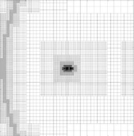
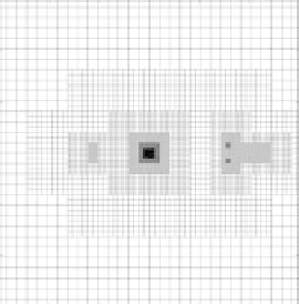
Fig. 1. Mesh obtained at the end of the 2-D CASIM simulation for a Halley-type comet.
(a)-(d) showing the progression of the grid refinement. The nucleus can be seen in the
center of (d). Note that (a) shows only a part of the more extended computational
domain.
restriction and interpolation functions to be used in these situations. For
CASIM3D, restriction is done using simple averaging of data at cell center.
Interpolation is performed using bilinear interpolation with a MUSCL-type
limiter (see Ref. 16).
3. Modeling of a Halley-Type Comet
In this simulation we consider a set of physical parameters globally con-
sistent with comet Halley's parameters as they were observed during the
1986 flybys. We only report in this paper the main variables that define