Geoscience Reference
In-Depth Information
21 22 23 24 25
16 17 18 19 20
11 12 13 14 15
678910
1
(a)
2345
x
(0) =
1
25
1
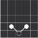
(b)
P
=
25
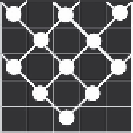
(c)
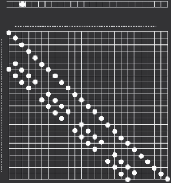
(d)
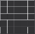
FIGURE 2.3
Generating a fractal using the generic diffusion model. (a) A 5 × 5 2D spatial system that can be
displayed as a 25 cell 1D system as shown in (d). (b) The generator in the 2D system. (c) The generated pattern
in the 5 × 5 system. (d) The matrix form of the CA model.
We have of course to make the dimensions of the model the same as that of the system so our
example is now much reduced in size to 25 cells. These cells are numbered in the square grid in
Figure 2.3a and we show the generator associated with the starting cell in Figure 2.3b. Note that the
starting cell is cell 3 and the generation of new cells which are switched on is at the northwest and
northeast of the initial cells 3, 7 and 9. In Figure 2.3c, we show the complete generation of the tree
for the 5 × 5 system. Now the starting vector of cells
x
(0) that are switched on - just cell 3 - is shown
at the top of Figure 2.3d, and below this is the matrix
P
where the main diagonal is set as positive
(i.e. 1) and the cells that get switched on for each cell considered are given by the dots below. The
way to interpret this is to look down each column which corresponds to a cell, and if there is a posi-
tive dot there, then the cell in question can be switched on but only if the vector
x
(0) is positive. This
operation is as follows: we take the row vector
x
(0) and multiply this by the matrix
P
, and if the main
diagonal of the matrix corresponds with a switched on cell in the vector, we look down the column
of the matrix and select those cells to be switched on which are positive.
This is hardly matrix multiplication, more a look-up table, and it is not stochastic in any way.
If we do this for the starting position, then as only cell 3 is positive, then column 3 is activated in
the matrix and the two cells in this column that correspond to those to be switched on are 7 and 9.
These duly get switched on in the new vector
x
(1) and then we consider how cells 3, 7 and 9 activate
their new neighbours. In this case, cell 3 acts in the same way but cells 7 and 9 activate 11, 13 and
15 which is the third row up in the tree structure in Figure 2.3c. And so the process continues in
building up trees, although in such a restricted space, we can only imagine the growing structures
across a much larger space. There are many variants we can consider. We can delete cells that are
already positive if we so specify a reaction, we can add new cells without taking into account any
considerations about neighbourhoods by using the exogenous driver and we can of course expand
the neighbourhoods to cover any areas of the space we want. In fact, the generic formulation gives
us all these possibilities, and in this sense, the reaction-diffusion framework is completely general.