Geoscience Reference
In-Depth Information
SR
WE
CWE
41
1
>3.8
>0.25
0
0
0
1000
200
km
PD
PE
>880
>20
0
0
Node range (cells)
1-100
100-300
301-882
0
10
20
30 40 Ma
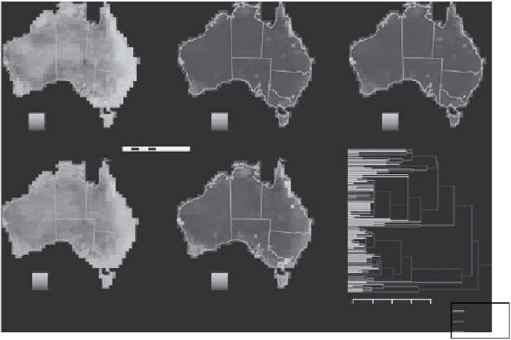
FIGURE 6.2
Geographic surfaces representing biodiversity indices for the Australian marsupials (SR, spe-
cies richness; WE, weighted endemism; CWE, corrected weighted endemism; PD, phylogenetic diversity; PE,
phylogenetic endemism). Spatial data are derived from IUCN distribution polygons (http://www.iucnredlist.
org), projected using an Albers equal area coordinate system and aggregated to 100 km cells. (Phylogenetic
data from Bininda-Emonds, O.R.P. et al.,
Nature
, 446, 507, 2007.)
A further step that can be applied to diversity analyses is to compare them against distributions
generated using null models. In the simplest case, one can assume a process of complete spatial
randomness (Diggle, 2003) at the cell level. Typically a systematic grid-based equivalent of some
random point pattern process mixing operation is applied, such that the species in each cell are ran-
domly reassigned to some other cell in the data set. This method of spatial disorganisation is a stan-
dard procedure that is used in most randomisation schemes in GC. However, improved null models
can be generated that mimic some aspect of the geographic structure of the distributions, applying
a more realistic and generally more conservative null model. For example, Laffan and Crisp (2003)
applied three randomisations. In the first model, the species were allowed to occur anywhere on the
landscape (i.e. a random distribution model). The second model applied the additional constraint
that the SR of each cell in the null distribution was forced to match that of the original data set
exactly. In the third model, the species distributions were further constrained to occur in a circular
distribution around a randomly selected seed point. The second and third models both required the
addition of an optimisation function to achieve the richness targets, in the form of an iterative swap-
ping algorithm. Other models, such as random walks or where species disperse analogously to a
drop of water on a sheet of paper (Jetz and Rahbek, 2001), can be implemented as functions of geo-
graphic proximity. Greater biological complexity can be incorporated using stochastic geographic
evolution models (Tello and Stevens, 2012), where species distributions are generated by stochastic
processes of lineage divergence, extinction and geographic range shifts. Such increasingly biologi-
cally realistic models are possible within tools like Biodiverse (Laffan et al
.
, 2010).
6.3.2 g
eneraliSed
d
iSSiMilarity
M
odelling
Diversity analyses require good-quality survey data. However, it not possible to conduct detailed
surveys everywhere (Rondinini et al., 2006). We can, however, attempt to predict the rate of change