Detection and measurement of wave breaking - Breaking and Dissipation of Ocean Surface Waves - page 81

55 s
( Figures 3.4 c-d are a zoom-in of Figures 3.4 a-b). In both Figures 3.4 a and 3.4 b, there are
well-defined peaks in the acoustic noise level associated with the breaking events. This
is in qualitative agreement with laboratory results by Melville et al. ( 1992 ). In contrast
to laboratory breaking waves, different fractions of energy are apparently lost by field
breakers, and therefore the breaking noise impact above the background in situ ambi-
ent noise is not always evident in field acoustic time series. For instance, the breaking
event that was observed visually at t

Figures 3.4 a-d plot time series of the digitised acoustic signal near t = 1 s and t =

53 s is not well defined in the time series in
Figure 3.4 b. It is, however, clearly seen in the corresponding acoustic noise spectrogram in
Figure 3.5 .
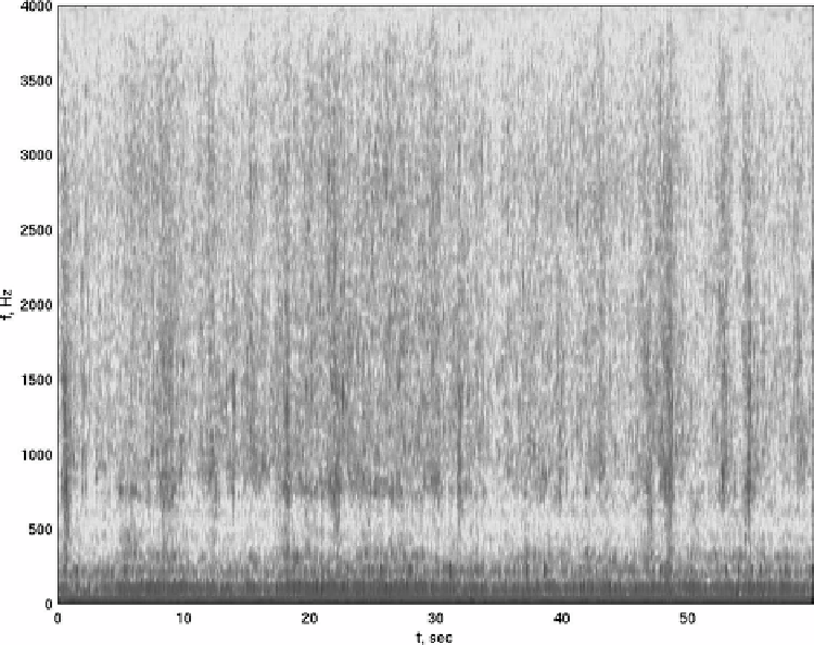
Figure 3.5 shows a spectrogram of this minute of the acoustic record. The spectrogram is
a time series of consecutive spectral densities computed over 256 readings of the acoustic
signal with a 128-point overlap; the segments were windowed with a Hanning window (see
Babanin et al. , 2001 , for further details). Values of the spectral density are shown using a

=

Figure 3.5 Spectrogram of one-minute record of acoustic noise recorded by a bottom-mounted
hydrophone during wave record 4 of Table 5.2 . Darker crests correspond to dominant waves break-
ing. The breaker in t = 1 s is depicted in Figures 3.2 and 3.4 a,c, and the breaker in t = 55 s in
Figures 3.3 and 3.4 b,d. Figure is reproduced from Babanin et al. ( 2001 ) by permission of American
Geophysical Union