Geoscience Reference
In-Depth Information
s
+
i
∞
+
∞
w
(
x
,
z
,
t
)=
∂
F
∂
1
=
−
d
p
d
k
z
4
π
2
i
−
∞
s
−
i
∞
cosh(
kz
)
g
k
tanh(
kz
)
p
2
p
exp
{
pt
−
ikx
}
−
×
H
(
p
,
k
)
,
(2.59)
cosh(
kH
)(g
k
tanh(
kH
)+
p
2
)
where
H
(
p
,
k
)=
∞
+
∞
d
t
d
x
exp
{−
pt
+
ikx
}
η
(
x
,
t
)
.
0
−
∞
In the case of arbitrary motion of the basin floor the solution of the problem
involves a cumbersome procedure—the calculation of a fourfold integral. Therefore,
for physical interpretation of the obtained integral representations it is expedient to
select several concrete versions of function
η
(
x
,
t
). This will permit to calculate
a large part of the integrals analytically.
Consider the following three types of deformation of the basin floor:
1. A linear (in time) displacement
τ
−
1
,
η
L
(
x
,
t
)=
η
θ
−
θ
−
θ
0
(
(
x
+
a
)
(
x
a
))
(
t
)
t
(2.60)
2. Running displacement
η
R
(
x
,
t
)=
η
0
(
θ
(
x
)
−
θ
(
x
−
b
)) (1
−
θ
(
x
−
vt
))
,
(2.61)
3. Harmonic oscillations of the basin floor
η
osc
(
x
,
t
)=
η
0
(
θ
(
x
+
a
)
−
θ
(
x
−
a
)) sin(
ω
t
)
(2.62)
where
is the Heaviside
function, 2
a
and
b
are the horizontal dimensions of the source. In all cases we con-
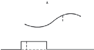
sider the rectangular distribution of deformations of the basin floor. The scheme
of motions of the basin floor in the case of a running displacement is shown in
Fig. 2.10.
For the tsunami problem the linear displacement itself has no physical
significance—it is useful only as a mathematical model. But from the function
η
0
is the amplitude of the basin floor displacement,
θ
Fig. 2.10 Model of running
displacement of basin floor