Geoscience Reference
In-Depth Information
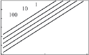
Fig. 5.3 Distance of disper-
sive destruction of a tsunami
wave as function of period
T
and ocean depth (numbers
at curves). The dotted line
shows a distance equal to
the Earth's equator, as a mea-
sure of a limit distance, that
can be covered by a tsunami
wave
(s)
)
√
g
H
λ
(
ω
L
cd
=
√
g
H
)
.
(5.1)
−
C
gr
(
ω
The following approximate relation follows from formula (5.1), when
λ
H
:
H
2
L
cd
∼
λ
.
(5.2)
The dependence (5.1) is presented in Fig. 5.3. The periods of tsunami waves,
that vary within limits of 10
2
-10
4
s, are plotted along the
x
-axis. Calculations are
performed for different depths of the water column (numbers near the curves). The
dotted line in the figure shows the Earth's equator, indicating a measure of the limit
distance, which can be covered by a tsunami wave. For typical depths of the open
ocean the whole range of tsunami wave periods can be divided into two intervals.
'Short-period' waves (
T
<
10
3
s), for which the manifestation of dispersion may
turn out to be significant, correspond to the first interval. In the second interval
(
T
>
10
3
s), along routes not longer than the Earth's equator, no significant mani-
festation of dispersion will be observed. In those cases, when the wave periods ex-
ceed 100 s only slightly, the manifestation of dispersion will already be noticeable
at relatively short distances of the order of 100-1,000 km.
Similar estimation can be performed in the case of transformation of a wave
packet due to amplitude dispersion, arising as a consequence of non-linearity. Con-
sider a wave with a crest of height
A
. The propagation velocity of the cr
est will d
iffer
from the velocity of linear long waves, its value can be estimated as
g(
H
+
A
).By
analogy with the distance of dispersive destruction, we introduce the distance of
'non-linear destruction' of a wave,
λ
√
g
H
g(
H
+
A
)
L
cn
=
.
(5.3)
−
√
g
H
If
A
/
H
1, then the following approximate relation will be valid:
H
A
.
L
cn
∼
λ
(5.4)