Geoscience Reference
In-Depth Information
For definiteness, we shall further consider the distribution of pressure in space in
formula (4.22) to have a Gaussian form:
p
(
z
)=
p
0
exp
,
z
2
a
2
−
(4.25)
where
p
0
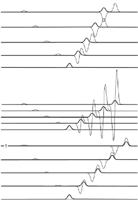
is the pressure amplitude. Figure 4.10 presents the example of the
movement of an atmospheric perturbation (in the region of a local enhancement
of pressure) and of the evolution of waves, generated by this perturbation. The
calculation is performed in accordance with formula (4.23) for three different ve-
locities of the perturbation. From the figure it is seen, that below the critical velocity
(
V
= 0
.
75), immediately under the atmospheric perturbation, a similar in shape,
Fig. 4.10 Profiles on free water surface of waves (thin line), formed by perturbation of atmospheric
pressure (thick lin
e), tr
avelling with a velocity
V
. The calculation is performed at
a
= 10 for fixed
time moments
t
g
/
H
= 0, 50, 100, 150, 200 (curves 1-5)