Geoscience Reference
In-Depth Information
140
∆
C
0
∆
t
Time
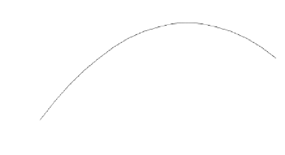
FIGURE 6.4
Visualization of the consequences of temporal discretization. Property evolves
within a time step, but values used to calculate flux do not.
being calculated. For the left face, we obtain
(
)
Q
>⇒
0
C
=
6
8
C
+
3
8
C
−
C
1
8
i
i
i
−
1
i
i
−
2
−
1
2
(
)
Q
<⇒
0
C
=
C
+
C
−
C
6
8
3
8
1
8
i
i
i
i
−
1
i
+
1
−
1
2
Using the Taylor series discretization described in the next paragraph, it can be
seen that, in the case of a regular discretization, advection calculated using this
approach is third-order accurate,
while pure upstream discretization is first-order
accurate and the linear approach (central differences) is second-order accurate. The
inconvenience of the QUICK discretization is that it requires additional approaches
close to the boundaries. This is not a very limiting factor in 1D calculation but it is
in 2D or 3D calculations, especially when the geometry is irregular.
1
6.2.3.2
Temporal Approach
In previous paragraphs, spatial discretization was analyzed. A solution was described
for the diffusion term and three discretizations were suggested for the advection
term but nothing was said about the time level at which the variables used to calculate
advection or diffusion are evaluated. Figure 6.4 shows an example of a time evolution
of a property
at a point. The curved line shows the continuous evolution and filled
circles show values at each time step. Vertical arrows show
C
C
values at the beginning
and end of a particular time step
∆
t
. The flux in that time step is proportional to the
product
. Values at the beginning and end of a time step are shown, as well as
concentration variation during that time step. The rate of accumulation at this point
is proportional to the slope of this line. The slope of this line also gives an idea of
the errors associated with the choice of
∆
C
∆
t
t
.
*


Search WWH ::

Custom Search