Geoscience Reference
In-Depth Information
V
i
V
i+1
V
i
−
1
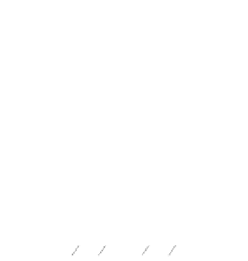
FIGURE 6.2
Example of one-dimensional (1D) grid.
simpler calculation is obtained if properties can be considered as being constant inside
the control volume and along parts of its surface. To make this possible without com-
promising accuracy, the control volume must be as small as possible; a fine-resolution
grid is needed.
In a 1D model, properties can be stored into 1D arrays (vectors). Adjacent
elements of a generic element
1 on the right
side (Figure 6.2). The length of a control volume must be small enough to allow
properties in its interior to be represented by the value at its center. In that case,
equations deduced in Section 3.2 apply and the rate of accumulation in volume
i
are
i
- 1 on the left side and
i
+
i
will
be given by
t
+
∆
t
t
(
VC
)
−
(
VC
)
Accumulation Rate
=
ii
ii
∆
t
where
is the time step of the model. This equation is simplified if the volume
remains constant in time. This is not the case in most coastal lagoons subjected to
changing winds and it is certainly not the case in tidal lagoons.
Exchanges between
∆
t
volume and neighboring ones are accounted for by advec-
tive and diffusive fluxes. Their calculation requires some hypotheses. Let us consider
Figure 6.2 and define the distances between the faces (spatial step) and the location
points where other auxiliary variables are defined as shown in
Figure 6.3.
The net
advective gain of matter to volume
i
i
is given by
(
)
*
tt
=
QC
−
QC
i
−
1
2
i
−
1
2
+
1
2
i
+
1
2
i
where
Qu
=
A
while the diffusive flux, using the approach of
Chapter 3,
is
1
2
1
2
1
2
i
−
i
−
i
−
given by
*
*
tt
=
tt
=
( )
( )
CC
x
−
+
CC
x
−
+
−
ν
A
i
i
−
1
+
ν
A
i
+
1
i
i
−
1
2
i
−
1
2
(
∆∆
x
)
i
+
1
2
i
+
1
2
(
∆∆
x
)
1
2
1
2
i
i
−
1
i
i
+
1


Search WWH ::

Custom Search