Geoscience Reference
In-Depth Information
Laptop
GPR system
LCD
display
DGPS receiver
DGPS
antenna
Keyboard
200-MHz
GPR antenna
fIGURe 26.5
The University of Tennessee Mobile GPR system. (From Freeland, R. S., R. E. Yoder, J. T.
Ammons, and L. L. Leonard, 2002,
Appl. Eng. in Agric
.. 18:647-650. With permission.)
30
25
20
15
10
5
0
0
1
2
3
4
Time (hr)
fIGURe 26.6
Water application rate (mm/hr) within 8 m diameter inner ring.
Water application
area
60-m dia.
90 min.
135 min.
180 min.
225 min.
0 min.
45 min.
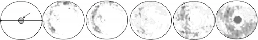
fIGURe 26.7
Top-down view of an ≈5 cm thick horizontal slice immediately atop the alluvium interface
depicting movement from the initial state (a) in 45 min sequential steps (b-f). Plot diameter is 60 m.
geospatial coordinates (latitude, longitude, elevation) with indexing pointers to their corresponding
scans within the GPR file. The spherical-projected GPS coordinate units (degrees) are transformed
to a flat-surface projection coordinate system (feet, meters), either State Plane or Universal Trans-
verse Mercator (UTM). The locations of each scan recorded between the GPS 1 sec position updates
are calculated using a linear series best-fit trend Microsoft EXCEL function (Microsoft Corp., Red-
mond, WA). Thus, each GPR sample value has corresponding three-dimensional spatial coordi-
nates for kriging. For any constant depth value, a horizontal plane can be interpolated and saved
in graphical file format. Multiple horizontal planes can be imported into a number of commercial
three-dimensional visualization packages (Figure 26.8) (e.g., open source MicroView, GE Health-
Care, Waukesha, WI). Stacked in sequence, the horizontal planes form a three-dimensional block.