Geoscience Reference
In-Depth Information
25.2.3 s
of i l
w
a t e R
c
o n t e n t
P
R o f i l e s
As a comparison bases for the GPR signal analysis, we numerically generated two-dimensional
soil water content profiles assuming a heterogeneous soil water distribution according to results
from earlier studies on homogeneous sand packages (Schmalz et al., 2003). Numerical experiments
were conducted using the Hydrus-2D software package of Simunek et al. (1996) to obtain two-
dimensional views of the infiltration and redistribution process. The Windows-based Hydrus-2D
package solves the Richards equation for variably saturated flow numerically, assuming applicabil-
ity of the van Genuchten-Mualem soil hydraulic functions.
Because of the geometric features of the sand tank, only flow in one particular cross section was
considered. To run Hydrus-2D, we implemented a relatively fine numerical mesh involving 4488
nodes depicting the geometry of the sand tank. An atmospheric boundary condition accounting for
infiltration and evaporation was imposed at the soil surface, whereas a seepage face was used at the
bottom boundary between the sand and a gravel drainage layer.
A heterogeneous soil water distribution could be depicted by assuming a spatially noncorrelated
distribution of the θ(
h
) a nd K(
h
) relations as measured in situ in eight depths with soil hydraulic probes.
The saturated hydraulic conductivity was assessed from the grain distribution using Hazen's empiri-
cal formula (Hölting, 1996) and was found to vary from 0.3 to 0.47 mh
−1
over the entire profile.
25.3
ReSUltS
25.3.1 w
a t e R
f
R o n t
P
R o P a g a t i o n
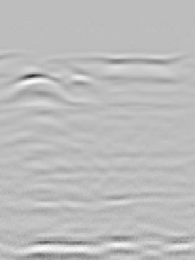
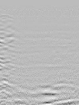
The processed GPR profiles (prior migration) allowed the clear identification of the penetrating
water front in infiltration experiments, especially when difference radargrams of two subsequent
time steps were computed (Figure 25.2a and Figure 25.2b). Difference radargrams are generated by
Offset (m)
Offset (m)
0.5
1.0
1.5
2.0
2.5
0.5
1.0
1.5 .0
2.5
0
0
10
10
A
D
20
20
30
30
B
40
40
A
B
C
C
Difference Plot of Two Timesteps
Difference Plot of Two Timesteps
(a)
(b)
fIGURe 25.2
Difference radargrams (nonmigrated) of the radargrams 3 and 2.45 (a) and 13 and 12.45
(b) hours after onset of irrigation. A marks the water front, B the electrode grid in 2 m depth, C the concrete
bottom in 2.5 m depth, and D is a highlighted artefact of a diffraction hyperbola caused by an electrode for
geoelectric measurements not mentioned in this paper.