Geoscience Reference
In-Depth Information
EM-38 (Geonics Ltd., Mississauga, Ontario, Canada) mounted on a nonmetallic cart that was pulled
through the field with a four-wheeled all terrain vehicle. The EC
a
values were recorded with a data
logger every second (1.5 m), and the location was geo-referenced using a Trimble GPS (Trimble
Navigation, Sunnyvale, CA) that was differentially corrected to provide an accuracy of <1 m.
Survey data were analyzed using the ESAP-95 software package (Lesch et al., 2000). The
ESAP-95 software package assesses the spatial dependency of the data, calculates soil sampling
locations that best encompass the variability present in the field, and uses measured soil data from
those locations and a stochastic calibration model to predict the spatial pattern of secondary soil
properties. Soil properties measured were 1:1 soil:distilled water electrical conductivity (EC
1:1
) and
pH (Smith and Doran, 1996), clay content (Kettler et al., 2001), and 2
M
KCl extractable NO
3
-N
(Keeney and Nelson, 1982). The EC
a
survey data and the output files of predicted secondary soil
properties were used to generate spatial maps by kriging using the GS+ software package (Robert-
son, 2000).
11.3 ReSUltS And dISCUSSIon
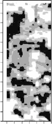
Apparent electrical conductivity values ranged from 45.5 to 81.1 mS m
−1
and were spatially depen-
dent (Figure 11.1). The spatial dependence in EC
a
was best fit with a spherical model (r
2
= 0.91,
residual mean square (RSS) = 26.9). Areas of the field exhibiting high EC
a
values were slightly
higher in elevation and had been subjected to erosion (tillage, wind, and water), and a portion of the
topsoil had been lost. Areas of the field exhibiting low EC
a
values tended to be depositional areas
of the field.
The correlation between EC
a
and EC
1:1
was not strong (r
2
= 0.22), likely because there was a
small range of EC
1:1
values (0.27 to 0.45 dS m
−1
) in these nonsaline soils. Bulk soil EC
a
is affected
by a number of soil properties including depth of topsoil, clay content, water content, and salt con-
tent (Rhoades and Corwin, 1990; Johnson et al., 2001). Laboratory EC
1:1
is more strongly correlated
with dissolved salts. In spite of the weak correlation between EC
a
and EC
1:1
, the predicted EC
1:1
map
(Figure 11.2) is visually similar to that for EC
a
(Figure 11.1). The spatial dependence predicted for
EC
1:1
was best fit with a spherical model (r
2
= 0.91,
RSS = 1.9E
−8
).
Clay content varied twofold (range 279 to
797 g kg
−1
) and was strongly correlated with
EC
a
(r
2
= 0.92). Others have also demonstrated
a strong correlation between EC
a
and clay con-
tent (Kitchen et al., 2003). As noted above, high
clay content was related to landscape position.
Predicted clay content was best described by an
exponential model (r
2
= 0.81, RSS = 46.7). Pre-
dicted clay content was positively correlated with
EC
a
with areas predicted to have a high clay con-
tent (Figure 11.3) being areas exhibiting high EC
a
values (Figure 11.1).
Soil NO
3
-N values ranged from 0.7 to 24.7
g kg
−1
and were correlated with EC
a
values (r
2
=
0.86). In these nonsaline soils, NO
3
-N is a major
anion, and EC
a
has been shown to have great
potential in monitoring NO
3
-N dynamics dur-
ing the growing season (Eigenberg et al., 2002).
The correlation between predicted NO
3
-N and
EC
a
was negative with low NO
3
-N values in areas
of the field (Figure 11.4) exhibiting high EC
a
4466032
4465834
4465635
4465436
4465238
620230
620389
620548
East
fIGURe 11.1
Spatial map of soil apparent elec-
trical conductivity for the study site near Bruning,
NE. ■ >72,
■
72 to 68,
■
68 to 64,
<64 mS m
−1
.