Geoscience Reference
In-Depth Information
1
1
a
F
(
X
)
Φ(
Z
)
0
0
−1
0
Z
X
=
y
(
Z
)
1
1
b
1−
m
Φ(
b
)
F
(
X
)
0
0
0
1
−1
0
b
X
=
y
0
(
Z
)
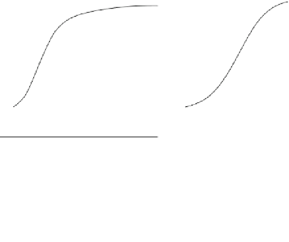
Fig. 12.38 Graphical representation of the transformation
ˈ
in
X
¼
ˈ
(
Z
). Distribution functions
ʦ
(
Z
) on the right-hand side are for standard normal random deviates. A value
F
(
X
) on the left-
hand side of (a) is equal to
(
Z
); (b) Shows the distribution function of a binary
random variable which can also be related to a standard normal random variable (Source:
Agterberg
1981
, Fig. 6)
ʦ
(
Z
)if
X
¼
ˈ
B
0
where
A
is the
original pattern and
B
0
an operator set consisting of two points. One point is the
origin of
B
and the other point occurs at a distance in the direction
The geometrical covariance
K
ʱ
(
h
) satisfies
K
ʱ
(
h
)
¼
mes
A
ʘ
. The accent on
B
denotes reflection of
B
with respect to its origin.
K
ʱ
(
h
) is shown in Fig.
12.40
for
the east-west direction. These measurements were obtained on the Quantimet
720 with linear correlator module at the Ecole Polytechnique in Montreal
(Agterberg and Fabbri
1978
). In order to obtain the corresponding statistical
covariance, the values of Fig.
12.40
were first increased by the factor mes
T
0
/mes
T
0
ʘ
ʱ
B
0
where
T
0
represents a square study area around
A
which measures exactly
80 km on a side. The statistical covariances were obtained by subtracting
m
2
from
the corrected geometrical covariances where
m
mes
A
/mes
T
0
is the proportion of
the study area underlain by acidic volcanics. The statistical covariances were
divided by the variance
C
0
¼
¼
m
2
and this gave the autocorrelation coefficients
plotted along the vertical axis with logarithmic scale in Fig.
12.41
. The signal-plus-
noise model with
r
h
¼
m
c
p
|
h
|) with
c
¼
0.87 and
p
¼
exp (
0.194 provides a
reasonably good fit.


Search WWH ::

Custom Search