Geoscience Reference
In-Depth Information
Log
10
E(k)
0.5
Log
10
k
0.25
0.5
0.75
1
1.25
1.5
1.75
−0.5
−1
−1.5
−2
−2.5
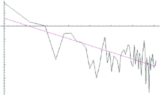
Fig. 12.37 Pulacayo zinc spectrum according to Lovejoy and Schertzer
(2007
, Fig. 3b). Red line
is theoretical with slope
K
(2) + 2
H
¼1.12;
K
(
q
) is “second characteristic function”;
K
(2) ¼0.05 was determined by double trace moment analysis; deviation from conservation
H
¼0.090 was derived from first order structure functions (Source: Lovejoy and Schertzer
2007
,
Fig. 3b)
ʲ
¼1
to the “hanning” method (Blackman and Tukey
1958
). In a discussion of this result,
Tukey (
1970
) pointed out that the resulting spectrum “drooped” although it was
within the 90 % confidence interval around the theoretical spectrum for the signal-
plus-noise model with negative exponential autocorrelation function. Re-plotting
the earlier results on a log-log plot shows a linear pattern with straight line of best fit
yielding
0.79. Although the straight-line model provided a good fit in this
plication, this estimate of
ʲ
¼
ʲ
is somewhat less than that obtained by Lovejoy and
Schertzer (
2007
).
12.8 Cell Composition Modeling
In various geomathematical applications to map data, the study area is subdivided
into square cells belonging to a regular grid. If random variables are defined for
such cells it is of interest to know how the parameters of these variables depend on
cell size. In 3-D applications the theory applies to blocks instead of grid cells. The
relationship between block values and block size has been considered by Matheron
(
1976
). One of his models (the discrete Gaussian model) is taken as a starting point
for most applications in this section. Some frequency distributions have the prop-
erty of “permanence”. This concept resembles that of limit distributions for sums of
independent random variables. Six types of permanent random variables were
considered in Agterberg (
1984
) where further discussions can be found. Only
Search WWH ::

Custom Search