Geoscience Reference
In-Depth Information
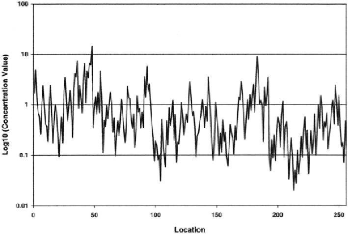
Fig. 12.19 Computer simulation experiment of Fig.
12.17
repeated after replacing dispersion
index
d
¼
0.4 by normal random variable
D
with
E
(
D
)
¼
0.4 and
σ
(
D
)
¼
0.1. Overall pattern
resembles pattern of Fig. 12.19 (Source: Agterberg
2007a
, Fig. 3)
X
1
/
Xn
2
were calculated for gold,
where
X
1
is the concentration value of a till sample with volume
V
1
that is randomly
located within a cell belonging to the grid of cells shown in Fig.
12.11
with
concentration value
X
n
cell size
V
n
. Figure
12.19
is a lognormal
Q
-
Q
plot of these
290 relative Au concentration values. The straight line provides a good fit except on
the left side of Fig.
12.19
where there is some bias related to the Au detection limit
and at the ends where frequencies of relative gold concentration values are small.
The logarithmic variance derived from the straight line of Fig.
12.19
is 0.5717.
This illustrates that positive skewness of the relative gold concentration values is
significant. Setting
V
n
/
V
1
equal to 2
20
yields an estimated value of
Relative element concentration values
Y
1n
¼
ʱ
*
¼
0.04124.
to
h
2
The logarithmic variance of
Y
12
would amount
0.03009.
Because it can be assumed that
Y
12
, like
Y
1n
, has lognormal distribution, its variance
is estimated to be
¼
0.5717/19
¼
2
(
Y
12
)
0.2326. Because this value is rather small,
Y
12
is
approximately normally distributed with standard deviation
σ
¼
σ
(
Y
12
)
¼
0.482. It fol-
lows that mean deviation from
E
(
Y
12
)
0.39. This would be a
crude estimate of average dispersion index in the random-cut model. It is close to
d
¼
1 amounts to m.d.
¼
0.43 estimated for the original logbinomial model of de Wijs (Table
12.2
).
Although m.d. and
d
are different parameters one would expect them to be
approximately equal to one another because of convergence of logbinomial and
lognormal distributions for increasing number of subdivisions (
n
). It was attempted
to repeat the preceding analysis for As but the 290 values
Y
1n
¼
¼
X
1
/
Xn
2
for As do not
show a simple straight line pattern, and m.d. could not be estimated with sufficient
precision (Figs.
12.20
,
12.21
,
12.22
, and
12.23
).
Search WWH ::

Custom Search