Geoscience Reference
In-Depth Information
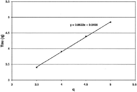
Fig. 12.15 Mass exponent
(
q
) plotted against relatively large values of
q
. Slope of best-fitting
straight line is used to estimate the dispersion index
d
¼
0.433 for gold (Source: Agterberg
2007a
,
Fig. 12)
˄
12.5 Other Modifications of the Model of de Wijs
The following one-dimensional computer simulation experiment for the model of
de Wijs was previously described in Agterberg (
1994
). Suppose
ʼ
(
S
A
) represents
1
. A line segment of length
L
can be
the measure of a set
S
in a segment of
ℜ
partitioned into
N
(
ʵ
) cells (intervals) of equal size
ʵ
; let
ʼ
i
(
ʵ
) denote the measure on
S
for the
i
-th cell of size
ʵ
in (0,
L
) with
i
¼
1, 2,
...
,
N
(
ʵ
). A simple stochastic
1
version of the multiplicative cascade model in
then is as follows. At the first
ℜ
stage (
k
¼
1) in a process of
n
stages, the interval (0,
L
) with measure
ʾ
L
is
subdivided into two equal intervals: (a) (0,
L
/2) with measure (1 +
B
)
ʾ
L
, and
(b) (
L
/2,
L
)with(1-
B
)
ʾ
L
, where
B
is a random variable with probabilities
P
(
B
0). At stage 2 these two intervals are halved again
with new measures for the halves defined in the same way as at stage 1. The process
is repeated at stages
k
¼
d
)
¼
P
(
B
¼
d
)
¼
1/2 (
d
>
...
At stage
k
the
i
-th subinterval with concentration
¼
3, 4,
L
/2
k
, and
E
{
X
i
(
value
X
i
(
ʵ
ʵ
¼
ʵ
¼
ʾ
) has size
)}
. The frequency distribution of
X
i
(
ʵ
ʵ !
0 and,
depending on the direction of ordering, slightly weaker than lognormal in both tails.
Figure
12.17
shows a realization of this process for
n
) is logbinomial, tending to become lognormal in the center as
0.4.
An obvious drawback of the original model of de Wijs is that, if the dispersion
index
d
applies at one stage, it is unlikely to apply at later steps because
d
generally
must be a random variable itself. In this section
d
will be replaced by the random
variable
D
.
¼
8,
ʾ
¼
1, and
d
¼
Search WWH ::

Custom Search