Geoscience Reference
In-Depth Information
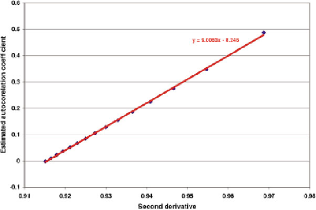
Fig. 11.14 Relation between estimated autocorrelation coefficients (
blue diamonds
) and second
derivative of corresponding continuous function. Best fitting straight line (
red
) is used for
extrapolation to the origin in Fig.
11.12
(Source: Agterberg
2012a
, Fig. 13)
Linear regression of the second derivative for
˄
(2) ¼0.979 on estimated values
resulted in the straight-line approximation shown in Fig.
11.14
. Although the
largest estimated autocorrelation coefficient that could be obtained by this method
is only 0.487 (for
k
¼
1), it now becomes possible to extrapolate toward much
smaller values of
k
h
, so that larger autocorrelation coefficients are obtained, by
using the second derivative on the right side of the preceding equation instead of the
second-order difference. The theoretical autocovariance function shown in
Fig.
11.12
was derived by transformation of the straight line of Fig.
11.14
for lag
distances with
h
¼
½
15), the curve of Fig.
11.12
(solid line) reproduces the estimated autocorrelation coefficients obtained by the
original multifractal model using second-order differences. Extrapolating toward
the origin by means of the second-order derivative results in an overall pattern that
closely resembles the hypothetical pattern of Fig.
6.19a
consisting of the nested
design of two superimposed negative semi-exponentials with a small white noise
component. Consequently, the multifractal autocorrelation model of Cheng and
Agterberg (
1996
), which is based on the assumption of scale-independence, con-
firms the existence of strong autocorrelation over short distances (
h
0.014 m. For integer values (1
k
<
2m).
11.4 Multifractal Patterns of Line Segments and Points
Multifractal case history studies presented earlier in this chapter were concerned
with chemical element concentration values in rocks and orebodies. In this section
the method will be applied to objects that are spatially distributed through a 2-D
Search WWH ::

Custom Search