Multifractals and Local Singularity Analysis - Geomathematics: Theoretical Foundations, Applications and Future Developments - page 426

1

0.8

0.6

0.4

0.2

0

-0.2

0 5 10 15 20 25 30

Lag distance (m)

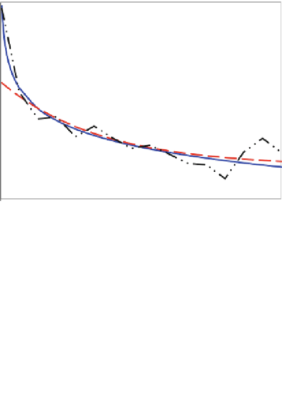
Fig. 11.12 Estimated autocorrelation coefficients (partly broken line) for 118 zinc concentration
values of Fig. 2.10 . Broken line represents best-fitting semi-exponential function used to extract
“signal” in Fig. 2.10 . Solid line is based on multifractal model that assumes continuance of self-
similarity over distance less than the sampling interval (Source: Agterberg 2012b , Fig. 3)

semivariogram model provides a good fit. It is equivalent to the logarithmic
semivariogram model introduced by Matheron ( 1962 , p. 180; also see Table 6.1 )
and also used by Agterberg ( 1994a , p. 226).
Cheng and Agterberg ( 1996 ) derived the following expression for the autocor-
relation function of a multifractal:

h i

ʵ ˄ ðÞ 2
2

2

C ʾ

Þ ˄ ðÞþ 1 Þ ˄ ðÞþ 1

2 k ˄ ðÞþ 1

ˁ k ðÞ ¼ ð k þ 1 þ ð k 1

˃

2

ðÞ ˃

2

ðÞ

where C is a constant, represents length of line segment for which an average zinc

concentration value is assumed to be representative,

E

˄ (2) is the second-order mass

2 (

exponent, ʾ represents overall mean concentration value, and ˃ ) is the variance

E

of the zinc concentration values. The unit interval is measured in the same

direction as the lag distance h . The index k is an integer value that later in this
section will be transformed into a measure of distance by means of k

ʵ

h .
Estimation for the 118 Pulacayo zinc values using an ordinary least squares
model with

¼ ½

˄

(2) ¼ 0.979 gave:

h i

1 : 979

2 k 1 : 979

1 : 979

ˁ k ¼

4 : 37 k ð þ 1 Þ þ ð k 1 Þ 8 : 00