Multifractals and Local Singularity Analysis - Geomathematics: Theoretical Foundations, Applications and Future Developments - page 425

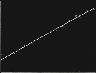
Fig. 11.11 Log-log plot for
relationship between ˇ 2 ( E )
and E (Source: Cheng and
Agterberg 1996 , Fig. 3)

1.8

1.4

1

0.6

0.2

−2 −1.8 −1.6 −1.4

Log e

−1.2 −1 −0.8

11.3.1 Pulacayo Mine Example

The Pulacayo orebody provides another example of application of multifractal spatial
correlation. The most important parameter on which this approach is based is the
second-order mass exponent

( 2 )(Fig. 11.11 ). In this application it is estimated by the
slope of the straight line fitted by least squares in Fig. 10.11 with

˄

0.019
( cf .Sect. 11.2.1 ). The semi-exponential autocorrelation previously used for smooth-
ing the zinc values of Fig. 2.10 is shown as a broken line in Fig. 10.12 together with
the autocorrelation coefficients (for lag distance h

˄ (2) ¼ 0.979

0) to which it was fitted. Its
nugget effect would explain about half of total variability of the zinc values. On the
other hand, use of the multifractal correlogram (solid line in Fig. 11.12 )showsa
continuous increase of spatial correlation towards the origin. The method used for
fitting the multifractal correlogram will be explained in more detail later in this
section. It does not apply when the lag distance becomes very small ( h

>

<

0.07 in
Fig. 10.12 ) so that the true white noise at the origin cannot be estimated by this
method. By means of local singularity mapping (Sect. 11.6.1 ), white noise will be
estimated to represent only about 2 % of total variability of the zinc values. It
represents measurement error and strong decorrelation at microscopic scale.
Figures 11.13a, b show the multivariate semivariogram previously shown

for the model of de Wijs (Fig. 11.10 ). It satisfies: ʳ k

ðÞ ¼ ʾ 2 ðÞ

h n o i

Þ ˄ ðÞþ 1 Þ ˄ ðÞþ 1

1
2

2 k ˄ ðÞþ 1

1 ð k þ 1 þ ð k 1 with ˄ (2) ¼ 0.979 and

2 (

ʾ 391.49 in comparison with experimental semivariogram values estimated

from the 118 Pulacayo zinc values using arithmetic and log-log scales. If

) ¼

E

(2) is
only slightly less than 1, the preceding theoretical equation can be approximated by
ʳ k

˄

as shown by Cheng and
Agterberg ( 1996 , Eq. 23). Figure 11.13c shows the experimental semivariogram
values on a graph with logarithmic scale in the horizontal direction only.
The straight line in Fig. 11.13c was fitted by least squares. The approximate

k ˄ ðÞ 1 ðÞ E ˄ ðÞ 1 log e

1
2

ðÞ ¼ ʾ 2 f ˄ ðÞþ 2 1 g˄ ðÞ 2