Geoscience Reference
In-Depth Information
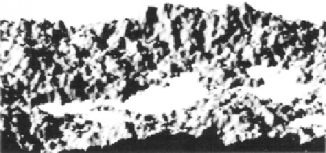
Fig. 10.1 Brownian
landscape after Mandelbrot
(1977, Plate 211)
intersected by horizontal
plane showing contours
with fractal dimension
D
¼1.5. Landscape below
this horizontal plane is not
shown (Source: Agterberg
1980
, Fig. 6)
dimensions. The problem of deposit size (metal tonnage) also is considered. Several
examples are provided of cases in which the Pareto distribution, which is closely
connected with fractals, provides good results for the largest deposits in metal
The dimension of a fractal is either greater than or less than the integer
Euclidian dimension of the space in which the fractal is imbedded. On the one
hand, fractals are often closely associated with the random variables studied in
mathematical statistics; on the other hand, they are connected with the concept of
“chaos” that is an outcome of some types of non-linear processes. An excellent
introduction to fractals and chaos in the geosciences is provided in Turcotte
(
1997
). Local singularity analysis (Cheng
2005
; Cheng and Agterberg
2009
)is
an example of non-linear modeling of geochemical data in mineral exploration
and environmental applications that produce new types of maps, which are
significantly different from conventional contour maps that tend to smooth
out local neighborhoods with significant enrichment of ore-forming and other
10.1.1 Earth's Topography and Rock Unit Thickness Data
Mandelbrot (
1977
) developed the novel approach for the modeling of irregular natural
phenomena as fractals characterized by their fractal dimension
D
.Hisfirstexample
consisted of measuring the length of the coastline of Britain (
D
1.3). Irregular curves
usually have a fractal dimension that exceeds the Euclidian dimension (
E
1) of a
straight line or geometric curve such as a circle satisfying an algebraic equation. Feder
(
1988
) pointed out that different coastlines have different fractal dimensions. For
example, the Australian coastline has
D
¼
1.1 but the Norwegian coastline with its
fjords has
D
1.52. Irregular surfaces have fractal dimensions exceeding
E
¼
2 but
their contours have 2
1. An example is shown in Fig.
10.1
that was generated as
follows (Mandelbrot
1977
, p. 207). A horizontal plateau was broken along a straight
line chosen at random to introduce a kind of vertical fault with a random difference
between the levels at the two sides of the fault plane. This process was repeated many
times resulting in the “ordinary” Brownian landscape of Fig.
10.1
. By “ordinary”
Mandelbrot meant that this landscape is closely related to the well-known process of
>
D
>
Search WWH ::

Custom Search