2-D and 3-D Trend Analysis - Geomathematics: Theoretical Foundations, Applications and Future Developments - page 249

a b

50

40

30

20

10

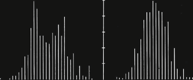
NATURAL LOGARITHM OF PER CENT COPPER

Fig. 7.10 (a) Histogram of natural logs of 516 copper values; (b) ditto for residuals from cubic
hypersurface; this curve is approximately Gaussian (Source: Agterberg 1974 , Fig. 51)

95-% confidence level. Consequently, it can be assumed that the cubic residuals of
the log-transformed copper values are indeed normally distributed.
A final example of 3-D trend analysis is for 335 Whalesback copper values from
20 holes drilled from the surface during an early stage of development of the
orebody. They are for an 800 ft. wide zone between 14,100 E and 14,900 E
which is 625 ft. deep. Figure 7.11 shows contours from the exponential cubic
hypersurface for copper on two levels together with an outline of the orebody
based on later information. Residuals for this hypersurface were shown in
Fig. 7.10b . Although the position of the central plane of maximum mineralization
in Fig. 7.11 is in close agreement with the outline of the orebody better results could
be obtained from the development holes drilled from the surface by using harmonic
trend analysis of the copper data as will be discussed in Sect. 7.4.2 .

7.2 Kriging and Polynomial Trend Surfaces

During the late 1960s, there was a considerable amount of discussion among earth
scientists and geostatisticians regarding the question of which technique is better:
trend surface analysis or kriging (see, e.g., Matheron 1967 )? The technique of
kriging (named after the South African geostatistician Danie G. Krige who first
applied regression-type techniques for gold occurrence prediction) is based on the
assumption of a homogeneous spatial autocorrelation function. If such a function
can be established independently, it can be used to solve the type of problem
exemplified in Fig. 7.12 . Within a neighborhood, values of a variable are known