2-D and 3-D Trend Analysis - Geomathematics: Theoretical Foundations, Applications and Future Developments - page 240

50,000 W 20,000 W

20.000 S

30.000 S

0.9

1.5

2.0

2.5

COMPLETE CUBIC SURFACE

3.0

HALF-CONFIDENCE INTERVAL

SCALE OF MILES

0 1 2 3 4 5

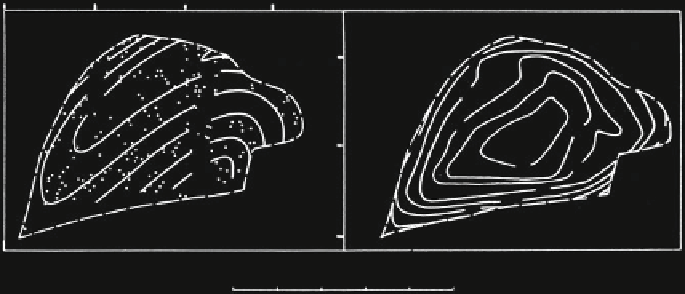
Fig. 7.4 Cubic trend surface for percent enstatite in orthopyroxene shown together with locations
of specimens and 95 % half-confidence interval (Source: Agterberg 1974 , Fig. 43)

boundary. It confirms the existence of the elongated ENE-WSW trending %Mg
minimum but not necessarily the maximum in the southeastern corner of the intru-
sion. As a further experiment, the original data set that consisted of 174 orthopyroxene
determinations was randomly divided into two interpenetrating subsets. The results of
trend surface analysis applied separately to these two subsets are shown in Fig. 7.5 .
The difference between the two cubic trend surfaces in Fig. 7.5 is less than 1 %Mg in
most of the Mount Albert peridotite intrusion.
There were 359 observation points for specific gravity. The quadratic surface is
not adequate for representing the trend of this variable. Cubic (ESS ¼ 39.9 %) and

quintic (ESS 56.0 %) trend surfaces are shown in Fig. 7.6 . The difference in

pattern between these two surfaces is caused mainly by the occurrence of a pocket
of practically unaltered peridotite in the eastern part of the body. The transition
from high-density to lower density material is relatively rapid and is poorly
approximated by the cubic.
A schematic contour map for elevation is given in Fig. 7.7a . A cross-section CD
was constructed and in Fig. 7.7b all observations within 2,500 ft. from the section
line were projected onto it. Then, average values for blocks measuring 5,000 ft. on a
side were calculated (Fig. 7.7e ). These block averages almost exactly coincide with
the intersection of the quintic trend surface with the cross-section CD. This shows
that: (1) the quintic trend surface provides a good fit to the specific gravity trend;
and (2) a trend surface also can be obtained by the relatively simple method of
moving averages. The method of moving or running averages consists of calculat-
ing arithmetic averages for a large number of overlapping blocks and contouring the
results. Obviously, this method can only be applied when there are many observa-
tions. If few observations are available, trend-surface analysis is to be preferred.
Because as many as 359 data points were available for specific gravity, 3-D trend
analysis also can be attempted by incorporating the elevation of each observation
point. The 3-D cubic trend equation contains 19 explanatory variables ( u , v , w , u 2 , uv ,
uw , v 2 , uw , w 2 , u 3 , u 2 v , u 2 w , uv 2 , uvw , uw 2 , v 3 , v 2 w , vw 2 ,and w 3 ) and 20 coefficients.
Its ESS-value amount to 55.1 % which is close to the previously mentioned

¼